
Mean, Median, Standard Deviation and Z-Scores Explained
Which average to report, why sample standard deviation divides by n - 1, why calculators disagree on quartiles, and how a z-score becomes a percentile.
· 9 min read
Descriptive statistics answer two questions about a pile of numbers: where is the middle, and how spread out is it? The answers look simple, but each one hides a choice. Mean or median? Divide by n or by n - 1? Which of nine quartile rules? This guide explains those choices with worked numbers you can reproduce in the Mean, Median and Mode Calculator, the Standard Deviation Calculator and the Z-Score Calculator.
Three averages and when each one is honest
The mean adds everything and divides by the count. It uses every value, which is its strength and its weakness. Take the data set 12, 15, 15, 18, 21, 22, 15, 25, 27, 30, 64. The sum is 264 over 11 values, so the mean is 24. Remove the 64 and the mean of the remaining ten drops to 20. One value moved the average by four units.
The median sorts the data and takes the middle one. Sorted, the set is 12, 15, 15, 15, 18, 21, 22, 25, 27, 30, 64, so the median is 21, the sixth of eleven values. Replace 64 with 640 and the median does not move at all. That is why house prices, household incomes and web page load times are usually reported as medians: a handful of extreme values would otherwise drag the mean away from anything typical. With an even count there is no single middle, so the median is the average of the two middle values, which may not be a value in the data.
The mode is the most frequent value. Here 15 appears three times, so the mode is 15. The mode is the only average that works for categories (the most common blood type, the most common answer on a 1 to 5 scale), and it can be plural: 3, 7, 7, 2, 9, 4, 4 has two modes, 4 and 7. When every value appears the same number of times there is no mode.
A practical rule: if the mean and median are close, the data are roughly symmetric and either works. If they are far apart, the data are skewed, and you should usually report the median for "typical" and the mean only when totals matter, such as total sales divided by stores.
Quartiles: why your calculator and your textbook disagree
Quartiles split sorted data into four equal parts. Q1 is the value a quarter of the way up, Q3 three quarters of the way up, and Q3 - Q1 is the interquartile range (IQR), the width of the middle half.
The trouble is that "a quarter of the way up" is ambiguous when the position falls between two data points. Rob Hyndman and Yanan Fan catalogued nine rules used by statistics packages in a 1996 paper, and four of them are common enough that students meet them:
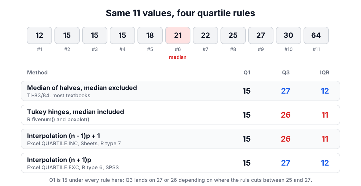
- Median of each half, median excluded. Split the data at the median, leave the median out and take the median of each half. This is what the TI-83 and TI-84 do and what most school textbooks teach.
- Tukey's hinges, median included. The same idea but the median goes into both halves when n is odd. R's
fivenum()andboxplot()use it. - Linear interpolation, inclusive. Q at position (n - 1)p + 1, interpolating between neighbours. This is Excel's QUARTILE.INC (and the older QUARTILE), Google Sheets, R's default type 7 and NumPy's default.
- Linear interpolation, exclusive. Position (n + 1)p. Excel's QUARTILE.EXC, R type 6, Minitab and SPSS.
For our 11 values, Q1 is 15 under every rule because the lower quarter is full of 15s, but Q3 is 27 under the first and fourth rules and 26 under the second and third. None of them is wrong. If your answer differs from the key, the method is the first thing to check; the calculator shows all four in one table.
Outliers and the box plot
John Tukey's rule draws two fences: Q1 - 1.5 x IQR and Q3 + 1.5 x IQR. With Q1 = 15, Q3 = 27 and IQR = 12, the fences are -3 and 45. The value 64 lies outside, so it is flagged. A box plot draws the box from Q1 to Q3 with a line at the median, extends whiskers to the most extreme values still inside the fences (12 and 30 here), and plots anything beyond as a separate point.
An outlier flag is a reason to look, not to delete. The most common causes are typos (a misplaced decimal), unit mix-ups (grams among kilograms) and genuinely unusual cases that are often the most interesting part of the data. Deleting values to make a chart look tidy is how results get quietly biased.
Standard deviation, and why n - 1
The standard deviation measures the typical distance from the mean. The recipe:
- Find the mean.
- Subtract it from each value to get the deviations.
- Square each deviation and add them up. This is the sum of squares.
- Divide by N for a population or by n - 1 for a sample. This is the variance.
- Take the square root.
The textbook set 2, 4, 4, 4, 5, 5, 7, 9 has mean 5. The squared deviations are 9, 1, 1, 1, 0, 0, 4 and 16, adding to 32. Divided by 8 that is 4, so the population standard deviation σ is 2. Divided by 7 it is 4.571, so the sample standard deviation s is 2.138.
Why the two versions? When you only have a sample, you measure deviations from the sample mean, and the sample mean is by definition the point that makes those deviations as small as possible. The true population mean is somewhere else, so deviations from it would be a little larger. Dividing by n - 1 instead of n inflates the estimate by just the right amount to cancel that bias on average. The fix is called Bessel's correction, and the "n - 1" is the degrees of freedom: once you know the mean and n - 1 of the deviations, the last deviation is fixed because they must sum to zero.
Use the population version only when the numbers really are the whole group you care about. In almost every practical case, from lab measurements to customer surveys, you want the sample version.
A note on precision
Many calculators and older spreadsheets use the shortcut variance = (Σx² - (Σx)²/n) / (n - 1). It is algebraically correct but numerically fragile. For readings such as 1000000.1, 1000000.2 and 1000000.3 the two terms are both around 3 x 10¹² and differ only in the digits that matter, so floating-point rounding can wipe out the answer or even make it negative. The calculator uses B. P. Welford's 1962 one-pass method, which updates the mean and sum of squares value by value, and it is tested against the NIST Statistical Reference Datasets built for exactly this problem. Those three readings correctly give s = 0.1.
Two useful companions
The coefficient of variation divides the standard deviation by the mean. A delivery time of 3 days ± 1 and an order value of $300 ± $20 cannot be compared in their own units, but their CVs (33% and 6.7%) can. The CV only makes sense for data on a true zero scale, so it is meaningless for temperatures in Celsius.
The standard error of the mean, s / √n, is not the spread of the data but the uncertainty of the average. For the test scores 72, 85, 90, 64 and 78 the standard deviation is 10.3 but the standard error is 4.6. Collect more scores and the standard error shrinks; the standard deviation does not. The standard error is what feeds confidence intervals, covered in the confidence interval and sample size guide.
Z-scores: putting values on a common scale
A z-score converts a value into "standard deviations from the mean":
z = (x - μ) / σ
A test score of 85 in a class with mean 70 and standard deviation 10 has z = 1.5. A score of 62 on a different test with mean 50 and standard deviation 8 also has z = 1.5, so the two performances are equally far above their averages even though the raw numbers differ.
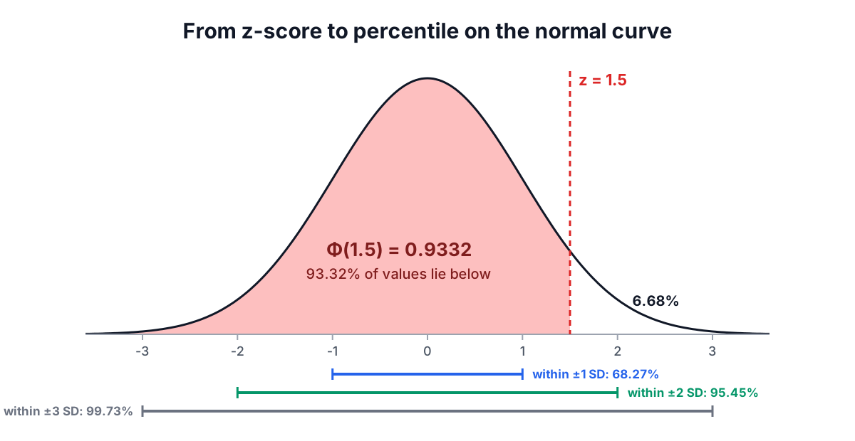
If the data are roughly normal, a z-score turns straight into a percentile through the standard normal cumulative distribution Φ(z). For z = 1.5, Φ = 0.9332, so the score beats about 93% of the group. The familiar empirical rule comes from the same curve: 68.27% of values lie within one standard deviation, 95.45% within two and 99.73% within three.
The reverse lookup is just as common. To find the score that marks the top 10%, find the z with 90% of the area to its left, which is 1.2816, and convert back: x = μ + zσ = 70 + 1.2816 x 10 = 82.8.
Where z-scores mislead
Percentiles from z-scores assume a bell-shaped distribution. Incomes, reaction times and file sizes are strongly right-skewed, and for them a z of 2 does not reliably mean the 98th percentile; the real share above it can be several times larger or smaller. If the data are skewed, rank them directly or use the median and IQR instead. Also make sure μ and σ describe the population you are comparing against: a z-score computed from a small sample's own mean and standard deviation can never be very large, because extreme values pull the standard deviation up with them (in a sample of n, no z can exceed (n - 1) / √n).
Precision matters in the tails. Many tools compute the upper tail as 1 - Φ(z), which loses every significant digit once Φ is within 10⁻¹⁶ of 1, so they report P(Z > 8) as 0. The calculator evaluates the tail directly and returns 6.22 x 10⁻¹⁶, which matters when you multiply a tiny probability by millions of events.
Choosing the right summary
For a quick, honest description of a data set, report the median and IQR when the data are skewed or contain outliers, and the mean and standard deviation when they are roughly symmetric. Always say which standard deviation you used, state the quartile method if anyone will check your numbers, and look at a box plot before trusting any single figure. Two very different data sets can share a mean and standard deviation; the picture is what tells them apart.