
Matrix Operations by Hand: Determinant, Inverse and Row Reduction
How row operations drive the determinant, inverse, rank and RREF, why order matters in matrix multiplication, and why exact fractions beat floating point on small matrices.
· 9 min read

Matrix calculations look intimidating because the grids are big, but almost everything a first linear algebra course asks you to compute comes down to one procedure: row reduction. The determinant, the inverse, the rank and the solution of a system of equations are all by-products of the same few row operations. Learn those operations and what each one does, and the rest is bookkeeping.
This guide covers the operations, the rules that decide when they are allowed, and why exact fractions matter more than you might expect. Every example can be reproduced, with the row operations shown, in the Matrix Calculator.
Shapes and the rules of combination
A matrix with m rows and n columns is called m×n. The shape decides which operations make sense.
Addition and subtraction work entry by entry, so both matrices must have the same shape. A 2×3 plus a 3×2 is undefined, not zero.
Scalar multiplication multiplies every entry by the same number. Multiplying by 1/2 halves everything.
Transpose swaps rows and columns, so a 2×3 becomes a 3×2. Row i of A becomes column i of Aᵀ.
Matrix multiplication is where most of the rules live. A×B is defined only when A has as many columns as B has rows, and the result has A's row count and B's column count. Each entry is a row of A dotted with a column of B. For
A = [1 2 3]      B = [ 7  8]
    [4 5 6]          [ 9 10]
                     [11 12]
the top-left entry is 1·7 + 2·9 + 3·11 = 58, and the full product is [58 64; 139 154], a 2×2 matrix. B×A, by contrast, is 3×3. Matrix multiplication is associative, (AB)C = A(BC), but it is not commutative: even for square matrices, A×B and B×A usually differ. Order matters whenever matrices represent steps applied one after another, such as rotate-then-scale versus scale-then-rotate in graphics.
Row operations: the engine behind everything else
There are three elementary row operations:
- Swap two rows.
- Scale a row by a non-zero number.
- Replace a row by itself plus a multiple of another row.
None of them changes the solution set of the system of equations a matrix represents, which is why they are allowed. Gaussian elimination uses them to clear the entries below each pivot, producing an upper-triangular form. Gauss-Jordan elimination keeps going: it scales each pivot to 1 and clears entries above it too, producing the reduced row echelon form (RREF).
In RREF, every non-zero row starts with a 1, each leading 1 sits to the right of the one above it, and every other entry in a pivot column is 0. Every matrix has exactly one RREF, however you choose to reach it, which makes it a reliable answer to compare against.
Solving a system
Write the coefficients and right-hand sides as an augmented matrix and reduce it. For
 2x +  y −  z =   8
−3x −  y + 2z = −11
−2x +  y + 2z =  −3
the augmented matrix [2 1 −1 8; −3 −1 2 −11; −2 1 2 −3] reduces in nine row operations to [1 0 0 2; 0 1 0 3; 0 0 1 −1]. Read the last column: x = 2, y = 3, z = −1. If a row reduces to [0 0 0 | 5], the system says 0 = 5 and has no solution. If a whole row reduces to zeros, one equation was redundant and there are infinitely many solutions.
Determinant and rank from the same reduction
The determinant of a square matrix is a single number that says whether the matrix can be inverted and how it scales area or volume. For a 2×2 matrix [a b; c d] it is ad − bc. For anything larger, cofactor expansion needs n! terms (720 for a 6×6), so in practice you row-reduce instead and track what each operation does:
- Swapping two rows flips the sign of the determinant.
- Scaling a row by k multiplies the determinant by k.
- Adding a multiple of one row to another leaves it unchanged.
Reduce to triangular form using only swaps and replacements, multiply the diagonal entries, and flip the sign once per swap. That is how the calculator computes it.
The rank is the number of pivots in the reduced form, which equals the number of linearly independent rows. The matrix [1 2 3; 4 5 6; 7 8 9] has rank 2: its third row is twice the second minus the first, so reduction leaves a row of zeros and the RREF is [1 0 −1; 0 1 2; 0 0 0]. A square matrix with rank below its size has determinant 0 and is called singular.
The inverse, and when it does not exist
The inverse A⁻¹ is the matrix with A × A⁻¹ = I, the identity. Only square matrices can have one, and only when the determinant is not zero.
To find it, place A beside the identity and row-reduce the whole block. When the left half becomes I, the right half is A⁻¹.
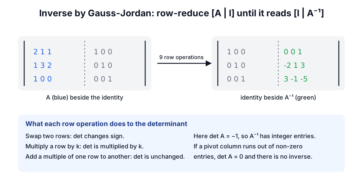
For A = [2 1 1; 1 3 2; 1 0 0] the determinant is −1, and the inverse is [0 0 1; −2 1 3; 3 −1 −5]. When the determinant is ±1 and every entry is an integer, the inverse is guaranteed to be all integers too, because the inverse equals the adjugate (a matrix of integer cofactors) divided by the determinant.
For a 2×2 matrix there is a shortcut: swap a and d, negate b and c, and divide by ad − bc. [1 2; 3 4] has determinant −2 and inverse [−2 1; 3/2 −1/2].
If the reduction runs out of non-zero entries in a pivot column, stop: the matrix is singular and no inverse exists. A good calculator says so plainly, with the rank, rather than returning a grid of enormous numbers. That grid is what floating-point software sometimes produces when rounding turns a true zero pivot into something like 1e-16 and then divides by it.
Why exact fractions matter on small matrices
Most calculators and spreadsheets use floating-point numbers, which store 0.1 and 1/3 as approximations. For everyday matrices the error is in the 15th digit and nobody notices. Two situations break that.
The first is singularity. A matrix whose determinant is exactly 0 can come out as 4e-17 in floating point, and the software then reports an inverse that is pure noise. With rational arithmetic the determinant is 0, and the matrix is reported as singular.
The second is ill-conditioning, where tiny input changes cause huge output changes. The classic example is the Hilbert matrix, whose entries are 1/(i + j − 1). The 3×3 case is
[ 1    1/2  1/3 ]
[ 1/2  1/3  1/4 ]
[ 1/3  1/4  1/5 ]
Its determinant is 1/2160 and its inverse is all integers: [9 −36 30; −36 192 −180; 30 −180 180]. Exact arithmetic returns exactly that. Floating point gets close for 3×3, but the error grows rapidly with size, and by around 12×12 a standard double-precision inverse of a Hilbert matrix is essentially meaningless.
The cost of exactness is that denominators can grow. A matrix typed with many decimals, such as 0.137, becomes 137/1000, and after a few row operations the fractions can get long. That is a display problem, not an accuracy one, and switching to decimal view rounds only the final answer. For matrices up to 6×6 the exact approach is fast enough that there is no reason to accept rounding.
A checklist for hand calculations
- Check shapes first. For A×B, the inner numbers in (m×n)(n×p) must match.
- Keep fractions as fractions. Converting 1/3 to 0.333 midway is the most common reason a hand-computed inverse fails its check.
- Verify the inverse. Multiply A by your answer; you should get the identity exactly.
- Use the determinant as an early warning. If it is 0, stop looking for an inverse and look at the rank instead.
- Do not assume AB = BA. Compute both if the order is not obvious from the problem.
Matrices sit next to plenty of other maths on this site. The Slope Calculator handles the single linear equation case, the Quadratic Equation Solver handles one non-linear one, and the Fraction Calculator is useful for checking a single row operation by hand.