Solving Systems of Linear Equations by Elimination, Step by Step

Elimination on the augmented matrix, Gauss-Jordan and row echelon form, spotting no solution or infinitely many, rank, determinants and Cramer's rule.

2026-10-29 · 10 min read

Illustration for the System of Equations Solver guide

A system of linear equations asks for values of several unknowns that satisfy several equations at once. Two equations in x and y are a staple of school algebra; three or four equations turn up in circuit analysis, chemistry, economics and almost every engineering course. Elimination is the method that scales: it works the same way for two equations as for two thousand, and it is what computer libraries run under the hood. This article goes through elimination by hand, the matrix form that makes it tidy, how to recognise systems with no solution or infinitely many, and where determinants and Cramer's rule fit in. Every example can be checked step by step with the System of Equations Solver.

The idea: make a variable disappear

Start with

2x + 3y = 7
 x −  y = 1

Multiply the second equation by 2 to get 2x − 2y = 2, then subtract it from the first: (2x + 3y) − (2x − 2y) = 7 − 2, which leaves 5y = 5, so y = 1. Substitute back into x − y = 1 to get x = 2. Check in the first equation: 2(2) + 3(1) = 7.

That is the whole method. You may add a multiple of one equation to another, multiply an equation by a non-zero number, or swap two equations, and none of these changes the solutions. You use those moves to remove one variable at a time until each equation has a single unknown.

Writing it as a matrix

Copying x, y and z on every line is wasted ink. The augmented matrix keeps only the coefficients, with the right-hand sides in a final column:

 x + y +  z =  6          [ 1  1   1 |  6 ]
     2y + 5z = −4    →    [ 0  2   5 | −4 ]
2x + 5y −  z = 27         [ 2  5  −1 | 27 ]

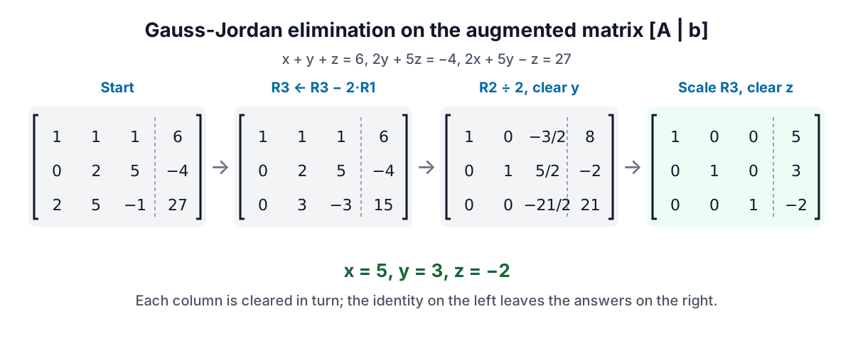
The three equation moves become row operations: swap two rows (Rᵢ ↔ Rⱼ), multiply a row by a non-zero number (Rᵢ ← k·Rᵢ), and add a multiple of one row to another (Rᵢ ← Rᵢ − k·Rⱼ). The goal is to make the left part look like the identity matrix, 1s on the diagonal and 0s elsewhere, at which point the last column is the answer.

Sequence of four augmented matrices for the system x plus y plus z equals 6, 2y plus 5z equals minus 4, 2x plus 5y minus z equals 27, showing row operations that clear the x column, then the y column, then the z column, ending at x equals 5, y equals 3, z equals minus 2

Worked through

The x column already has a 1 at the top. Clear the 2 below it with R3 ← R3 − 2·R1, giving row 3 = [0 3 −3 | 15].
Make the y pivot 1 with R2 ← R2 ÷ 2, giving [0 1 5/2 | −2].
Clear y from the other rows: R1 ← R1 − R2 gives [1 0 −3/2 | 8], and R3 ← R3 − 3·R2 gives [0 0 −21/2 | 21].
Make the z pivot 1 with R3 ← (−2/21)·R3, giving [0 0 1 | −2].
Clear z: R1 ← R1 + (3/2)·R3 gives [1 0 0 | 5], and R2 ← R2 − (5/2)·R3 gives [0 1 0 | 3].

The solution is x = 5, y = 3, z = −2. Substituting back: 5 + 3 − 2 = 6, 2(3) + 5(−2) = −4, and 2(5) + 5(3) − (−2) = 27.

Fractions such as 5/2 and −21/2 appear in the middle even though the answers are whole numbers. Working with exact fractions, as the solver does, means they cancel cleanly; working with rounded decimals can leave 4.9999999 where 5 should be.

Gaussian versus Gauss-Jordan

Gaussian elimination only clears the entries below each pivot, producing a staircase called row echelon form, then solves from the bottom row upward by back-substitution. Gauss-Jordan elimination also clears above each pivot and scales pivots to 1, producing reduced row echelon form (RREF), where the answers sit in the last column with nothing left to do. By hand, Gaussian elimination is usually less work; Gauss-Jordan is easier to read, which is why the solver shows it. The method is old: the Chinese text The Nine Chapters on the Mathematical Art, compiled around two thousand years ago, solves systems of three equations with counting rods arranged in exactly this tabular form.

One solution, none, or infinitely many

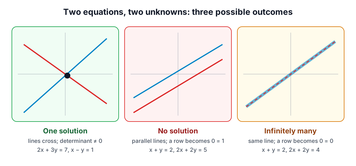
Every linear system has exactly one of three outcomes. For two unknowns, each equation is a line, and the picture says it all.

No solution

 x +  y = 2
2x + 2y = 5

R2 ← R2 − 2·R1 gives [0 0 | 1], that is, 0x + 0y = 1, or 0 = 1. No values can make that true, so the system is inconsistent. The lines have the same slope and different intercepts, so they are parallel. Whenever elimination produces a row of zeros on the left with a non-zero number on the right, stop: there is no solution.

Infinitely many solutions

 x + y +  z = 6
 x − y + 2z = 5
2x     + 3z = 11

The third equation is the sum of the first two, so it adds no new information. Elimination produces a row of all zeros, [0 0 0 | 0], which is always true and can be dropped. Two equations in three unknowns leave one unknown free. The RREF reads

x + (3/2)z = 11/2
y − (1/2)z = 1/2

so with z = t for any number t, the solutions are x = 11/2 − (3/2)t, y = 1/2 + (1/2)t, z = t. This parametric form is a complete answer: it describes a whole line of solutions in three-dimensional space. Setting t = 1 gives (4, 1, 1), which you can check satisfies all three original equations. The unknowns without a pivot are the free variables; the solver names them and writes the family with t, s, u as needed.

Rank: the test behind the three cases

The rank of a matrix is the number of pivots elimination finds, which is the number of genuinely independent equations. Compare the rank of the coefficient matrix A with the rank of the augmented matrix [A | b], and the number of unknowns n:

Condition	Outcome
rank A < rank [A \| b]	No solution (a row became 0 = non-zero)
rank A = rank [A \| b] = n	Exactly one solution
rank A = rank [A \| b] < n	Infinitely many, with n − rank free variables

This is the Rouché–Capelli theorem, and it works for any number of equations, including more equations than unknowns. An overdetermined system, say three equations in two unknowns, has a solution only if the extra equations agree with the others.

Determinants and Cramer's rule

For a square system (as many equations as unknowns), the determinant of the coefficient matrix gives a quick verdict: if it is not zero, there is exactly one solution; if it is zero, there is either none or infinitely many, and elimination tells you which.

For a 2 × 2 system ax + by = e, cx + dy = f, the determinant is D = ad − bc, and Cramer's rule gives

x = (ed − bf) / D        y = (af − ec) / D

In general each unknown equals Dᵢ / D, where Dᵢ is the determinant with that unknown's column replaced by the right-hand side. For the 3 × 3 example above, D = −21, Dx = −105, Dy = −63 and Dz = 42, so x = 5, y = 3 and z = −2, matching elimination.

Cramer's rule is elegant and handy as a check, which is how the solver uses it, but it is slow for larger systems: computing determinants by cofactor expansion takes on the order of n! operations, while elimination takes on the order of n³. For a 10 × 10 system that is millions of steps against a few hundred. The determinant itself is best found by elimination too: it is the product of the pivots, with a sign change for each row swap.

Practical tips

Rewrite in standard form first. Move all variable terms to the left and constants to the right: 3x = 2y + 1 becomes 3x − 2y = 1. The solver does this for you and shows the result.
Use a 1 as the pivot when you can. Swapping a row with a leading 1 to the top avoids fractions early on.
Clear fractions in the input. Multiply x/2 + y/3 = 4 through by 6 to get 3x + 2y = 24. It is the same equation with easier numbers.
Always substitute back. It takes a minute and catches nearly every arithmetic slip. The solver prints the substitution check for each equation.
Linear means linear. Terms like xy, x² or 1/x make the system non-linear, and elimination in this form does not apply.

Where systems come from

Mixtures and word problems: a café sells 120 drinks at $3 and $5 for $460 in total; x + y = 120 and 3x + 5y = 460 give x = 70 and y = 50.
Circuits: Kirchhoff's current and voltage laws give one linear equation per node or loop; the unknowns are currents.
Chemistry: balancing a reaction means solving for coefficients that conserve each element, usually a system with one free variable that you scale to whole numbers.
Economics and statistics: equilibrium prices, input-output models and the normal equations of least-squares regression are all linear systems.

For more than four unknowns, or for matrix operations such as inverses and products, use the Matrix Calculator. For a single equation with a squared term, the Quadratic Equation Solver is the right tool. And for any system of two to four linear equations, type them as you would write them into the System of Equations Solver and follow the row operations to the answer.

Sources

Gilbert Strang, Introduction to Linear Algebra, 5th edition, chapter 2 (elimination) and chapter 5 (determinants and Cramer's rule).
Gene H. Golub and Charles F. Van Loan, Matrix Computations, 4th edition, chapter 3, on the operation count of Gaussian elimination.
The Nine Chapters on the Mathematical Art, chapter 8 (Fangcheng, rectangular arrays), in the translation and commentary by Shen Kangshen, John N. Crossley and Anthony W.-C. Lun (Oxford, 1999).