
Cut and Fill Earthwork Volumes: Grid, End Area and Prismoidal
The borrow-pit grid method and how it splits transition cells, average end area versus the prismoidal formula for road sections, and how swell and shrinkage decide whether a site really balances.
· 11 min read

Every graded site, from a house pad to a highway, starts with the same question: how much soil has to be dug out, how much has to be placed, and does one cover the other? The answer depends on the survey data you have and the method you use to turn it into volume. This post explains the three methods built into the Cut and Fill Calculator, shows where each formula comes from, and covers the swell and shrinkage factors that decide whether a site really balances.
Depth of cut and fill at a point
Earthwork starts with two surfaces: the existing ground from a topographic survey and the proposed formation level from the grading design. At any point, the depth is:
h = existing level - proposed level
h > 0: cut      h < 0: fill
Proposed means formation level, the top of the subgrade, not the finished surface. If a car park has 75 mm of asphalt over 200 mm of base, the formation is 275 mm below the finished level, and the cut is measured to that.
The grid (borrow-pit) method
For pads and lots, the survey is a grid of spot levels at regular spacing. Each grid square is treated as a prism whose top is the ground and whose bottom is the proposed surface, so its volume is the plan area times the average of the four corner depths. Summing over the whole grid gives the classic borrow-pit formula:
V = A/4 x (Σh1 + 2Σh2 + 3Σh3 + 4Σh4)
where A is the area of one square and h1, h2, h3, h4 are the depths at points shared by one, two, three or four squares. Corners of the site count once, edge points twice, the inside corner of an L-shaped site three times, and interior points four times.
That works when a square is entirely in cut or entirely in fill. Squares that straddle the line where cut changes to fill need splitting, otherwise the cut and fill inside them cancel out and both totals come out too small. The four-point method handles these transition cells:
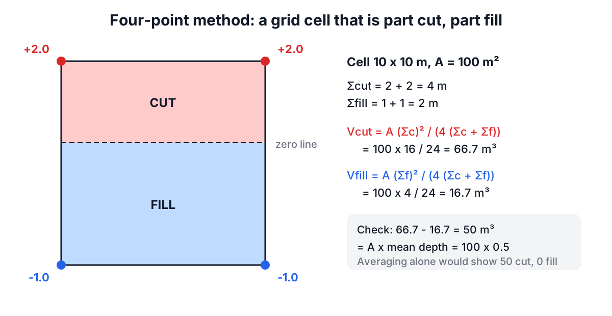
Vcut  = A x (Σc)² / (4 x (Σc + Σf))
Vfill = A x (Σf)² / (4 x (Σc + Σf))
Σc is the sum of the cut depths and Σf the sum of the fill depths at the cell's corners, both taken as positive. In the example, a 100 m² cell with corners at +2, +2, -1 and -1 m has 66.7 m³ of cut and 16.7 m³ of fill. Their difference, 50 m³, equals the area times the mean signed depth, so the net is preserved while both gross quantities are now counted. Gross quantities matter because you pay to dig the cut and to place the fill, not just for the difference.
On the calculator's default 4 x 4 grid at 10 m spacing, with ground falling from 101.2 m to 99.2 m and a pad at 100.2 m, the cut is 181.1 m³ and the fill 133.6 m³. Lowering the pad to 100.0 m raises cut to 296.7 m³ and drops fill to 69.2 m³. The colour map in the calculator shows which cells change, which is the fastest way to tune a pad level.
Cross-sections: average end area and the prismoidal rule
Roads, channels and embankments are surveyed as cross-sections at stations along a centreline. The designer plots the existing ground and the design template at each station and measures the cut area and fill area. Volume between two sections L apart is then:
Average end area:   V = L x (A1 + A2) / 2
Prismoidal:         V = L/6 x (A1 + 4 Am + A2)
The average end area method is standard in highway practice because it is simple and only needs the end sections. It is exact when the area changes linearly along the line, and it overestimates when a section shrinks to a point, as in a cut that tapers out: a pyramid computed by average end area comes out 50% too large. The prismoidal formula is exact for any prismoid, but needs the area Am at the midpoint. When sections are at equal spacing d and there is an odd number of them, alternate sections can serve as midpoints, and the formula becomes Simpson's rule:
V = d/3 x (A1 + 4A2 + 2A3 + 4A4 + ... + An)
For five sections 20 m apart with cut areas of 12.5, 8.2, 3.1, 0 and 0 m² and fill areas of 0, 1.5, 6.4, 11.8 and 7.2 m², average end area gives 351 m³ of cut and 466 m³ of fill, and the prismoidal rule gives 343 and 488 m³. Many contracts specify average end area for payment, so check which method governs before arguing over the difference.
Swell, shrinkage and the balance
Soil in the ground is at its bank (in-situ) density. Dig it and it loosens, so the volume in the trucks is larger: that increase is swell. Compact it in fill and it becomes denser than it was in the bank: that loss is shrinkage. Typical values are about 25% swell and 10 to 15% shrinkage for common earth, 30 to 40% swell for clay, and 50% or more swell for blasted rock, which may even bulk when placed in fill. A geotechnical report or test sections give site-specific figures.
loose volume       = bank x (1 + swell)
bank needed for fill = compacted fill / (1 - shrinkage)
surplus (bank)     = cut - bank needed for fill
A site with 181 m³ of cut and 134 m³ of fill looks like it has 47 m³ to spare. With 10% shrinkage, the fill needs 148.5 m³ of bank material, so only 32.7 m³ is really surplus, and at 25% swell that is 40.8 m³ to haul away. On the road example, 343 m³ of cut cannot supply 488 m³ of fill; with shrinkage the shortfall is 199 m³ of bank material to import. Ignoring shrinkage is the classic reason a "balanced" site ends up buying fill.
When the simple methods break down
- Coarse grids. The grid method assumes each square is a plane between its corners. Ridges, ditches and banks between survey points are invisible. Add spot levels at breaks of slope or use a triangulated surface model.
- Curved alignments. Average end area assumes sections are parallel. On tight curves, the centroid of each section travels a different distance, and a curvature correction is needed.
- Topsoil and unsuitable material. Topsoil is stripped and stockpiled separately and is not fill. Soft or organic soils dug from cut may not be reusable at all.
- Rock. Excavation in rock is priced differently and swells far more. Separate it from common excavation.
Modern practice computes volumes between two triangulated surfaces in civil design software, which is the same idea as the grid method with irregular triangles. The hand methods remain useful for checks, small sites and understanding what the software is doing.
Once the site is graded, the Asphalt Calculator and Asphalt Tonnage cover the paving, and the Gravel and Mulch Calculator handles base course. If your levels come from GPS points, the Coordinate Distance Calculator checks the spacing between them, and the Slope Calculator converts level differences to grades. Earthwork for structures, retaining walls and slopes steeper than about 1 in 3 needs a geotechnical engineer's input.