
Darcy-Weisbach and the Colebrook Equation: Pipe Friction Loss in Practice
Where the friction factor comes from, how to solve Colebrook and when Swamee-Jain is good enough, typical roughness and K values, and a full worked pressure drop.
· 12 min read

Pressure drop is the number that sizes pumps, decides pipe diameters and explains why the far end of a system is starved. The Darcy-Weisbach equation is the general method for it: it works for any Newtonian liquid, in any unit system, laminar or turbulent, as long as you have the right friction factor. This guide explains the equation and the friction factor behind the Pipe Pressure Drop Calculator, how the Colebrook equation is solved, when an explicit approximation is good enough, where typical roughness and fitting K values come from, and a fully worked example.
The Darcy-Weisbach equation
Friction loss along a straight, full, round pipe is:
Δp = f × (L / D) × (ρ v² / 2)
h_f = f × (L / D) × (v² / 2g)
- f is the Darcy friction factor (dimensionless)
- L and D are pipe length and inside diameter
- ρv²/2 is the dynamic pressure, v²/2g the velocity head
Read it as "a number of velocity heads per diameter of pipe". Henry Darcy measured water pipes in the 1850s and Julius Weisbach gave the equation its form a decade earlier. Because the loss scales with v², and v with 1/D², the loss at a fixed flow scales roughly with 1/D⁵. A modest increase in bore cuts friction dramatically, which is why pipe size is the most powerful lever on pumping energy.
A warning on names: the Fanning friction factor used in some chemical engineering texts is one quarter of the Darcy value. Mixing them gives a fourfold error. This guide and the calculator use Darcy (and display Fanning alongside).
The friction factor: laminar and turbulent
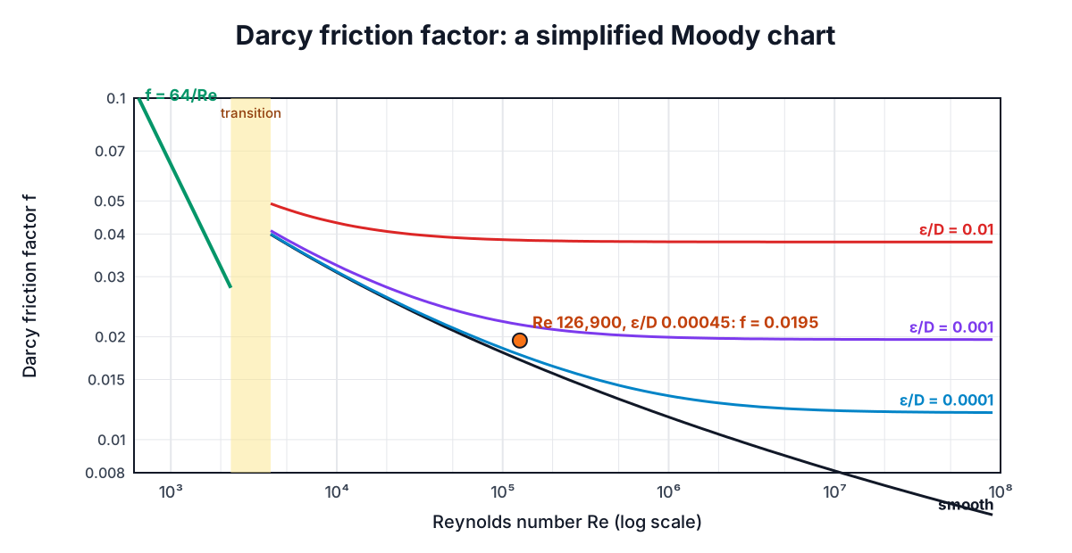
In laminar flow (Re below about 2300) the friction factor comes straight from the Hagen-Poiseuille solution:
f = 64 / Re
Roughness does not matter, and the pressure drop is proportional to viscosity and to flow, not flow squared.
In turbulent flow, f depends on both the Reynolds number and the relative roughness ε/D. Cyril Colebrook combined the smooth-pipe law of Prandtl and the fully rough law of von Kármán into one formula in 1939:
1/√f = −2 log10( ε/(3.7 D) + 2.51/(Re √f) )
Lewis Moody plotted it in 1944, giving the chart printed in every fluids textbook. The chart's left side is the laminar line, the right side flattens as the pipe becomes "fully rough" and f depends only on ε/D.
Solving Colebrook
f appears on both sides, so Colebrook has no closed-form answer in elementary functions. The usual approach is fixed-point iteration on x = 1/√f:
x_new = −2 log10( ε/(3.7D) + 2.51 x_old / Re )
Start anywhere sensible and it converges fast. For the example below (Re = 126,900, ε/D = 0.00045), starting from f = 0.02:
| Step | 1/√f | f |
|---|---|---|
| 1 | 7.16509 | 0.019479 |
| 2 | 7.15893 | 0.019512 |
| 3 | 7.15933 | 0.019510 |
| 4 | 7.15931 | 0.019510 |
Three steps already give four significant figures. The calculator iterates to a relative change of 10⁻¹² and reports how many steps it took.
Explicit approximations avoid iteration:
- Swamee-Jain (1976): f = 0.25 / [log10(ε/(3.7D) + 5.74/Re^0.9)]², within about 1 to 2% of Colebrook for 5,000 < Re < 10⁸ and 10⁻⁶ < ε/D < 10⁻².
- Haaland (1983): 1/√f = −1.8 log10[(ε/3.7D)^1.11 + 6.9/Re], similar accuracy.
For the example, Swamee-Jain gives 0.01960 (+0.45%) and Haaland 0.01927 (−1.2%). Those differences are tiny compared with the uncertainty in roughness, so any of them is fine for design. The calculator shows Colebrook and Swamee-Jain side by side so you can see that for yourself.
Roughness: the input you know least well
Typical absolute roughness for new pipe (from Moody and standard texts):
| Material | ε (mm) | ε (ft) |
|---|---|---|
| Drawn tubing, copper, PVC, PE | 0.0015 | 0.000005 |
| Commercial steel, wrought iron | 0.045 | 0.00015 |
| Asphalted cast iron | 0.12 | 0.0004 |
| Galvanized iron | 0.15 | 0.0005 |
| Cast iron, uncoated | 0.26 | 0.00085 |
| Concrete | 0.3 to 3.0 | 0.001 to 0.01 |
| Riveted steel | 0.9 to 9.0 | 0.003 to 0.03 |
These are for new pipe. Corrosion, tuberculation and scale can raise steel roughness by five to ten times over the years, and they also shrink the bore, which hurts even more. For long-life water systems many designers either use an aged roughness or apply a margin to the calculated head. In the example below, switching from new steel (0.045 mm) to uncoated cast iron (0.26 mm) raises the friction loss from 15.8 to 21.3 kPa, 35% more for the same flow.
Minor losses: fittings and valves
Every elbow, tee, valve, entrance and exit adds a loss proportional to velocity head:
Δp_minor = ΣK × ρ v² / 2
Typical textbook K values for turbulent flow:
| Fitting | K (typical) |
|---|---|
| 90° elbow, regular, flanged | 0.3 |
| 90° elbow, regular, threaded | 1.5 |
| 90° elbow, long radius, flanged | 0.2 |
| Tee, line flow / branch flow (flanged) | 0.2 / 1.0 |
| Gate valve, fully open | 0.15 |
| Globe valve, fully open | 10 |
| Ball valve, fully open | 0.05 |
| Swing check valve | 2 |
| Square-edged entrance from a tank | 0.5 |
| Exit into a tank | 1.0 |
Published values vary with size and manufacturer by as much as ±50%. The Crane Technical Paper 410 method ties K to pipe size through a friction factor for clean commercial steel, and the 2-K and 3-K methods add a Reynolds number term for low flows. When you have the valve maker's Cv or K, use it. You can also express a fitting as an equivalent length of pipe, L_eq = K D / f, but that hides the fact that f changes with flow.
Minor losses are often minor only in long pipelines. In a pump skid or a plant room, fittings can be most of the total.
Worked example
Water at 20 °C, 10 L/s through 100 m of 100 mm new commercial steel, with four flanged elbows and two open gate valves, inlet and outlet at the same level.
- Velocity: A = π × 0.1² / 4 = 0.007854 m², v = 0.01 / 0.007854 = 1.273 m/s.
- Reynolds number: ρ = 998.2 kg/m³, μ = 0.0010016 Pa·s, Re = 998.2 × 1.273 × 0.1 / 0.0010016 = 126,900. Turbulent.
- Relative roughness: ε/D = 0.045 / 100 = 0.00045.
- Friction factor: Colebrook gives f = 0.01951 (table above).
- Dynamic pressure: ρv²/2 = 998.2 × 1.273² / 2 = 809.1 Pa.
- Pipe friction: Δp_f = 0.01951 × (100 / 0.1) × 809.1 = 15,786 Pa = 15.79 kPa.
- Fittings: ΣK = 4 × 0.3 + 2 × 0.15 = 1.5, so Δp_m = 1.5 × 809.1 = 1,214 Pa.
- Total: 17.0 kPa, or 17,000 / (998.2 × 9.80665) = 1.74 m of head.
If the outlet were 10 m higher, add ρgΔz = 97.9 kPa of static head; the calculator has an elevation field for that. To find the pump power for this duty, carry the total head into the Pump Power Calculator.
Reading the system curve
Run the same pipe at different flows and plot the loss: you get the system curve. In turbulent flow it rises roughly with the square of flow (slightly less, because f falls as Re rises). Laying it over a pump's head-flow curve shows where the two meet, which is the operating point. Throttling a valve steepens the system curve; a variable speed drive shifts the pump curve instead, usually with far less wasted energy.
When this method does not apply
- Compressible gas flow with a pressure drop above about 10% of the inlet pressure: density changes along the pipe. Use an isothermal or adiabatic compressible-flow method.
- Two-phase flow (steam and condensate, gas and liquid): needs specific correlations.
- Non-Newtonian fluids such as slurries and sludges: need rheological models.
- The transition band, Re 2300 to 4000: f is genuinely uncertain. The calculator uses Colebrook there, the more conservative choice, and warns you.
- Partly full pipes and open channels: use Manning or similar.
The Hazen-Williams formula is still common in water distribution and fire protection design. It is fine for water near room temperature in turbulent flow but has no viscosity term, so it should not be used for hot water, oils or laminar flow. Darcy-Weisbach has no such limits. For the regime question, see the Reynolds number guide; for the energy balance that ties losses to pressures and heights, see Bernoulli's equation with worked examples.