
How to Do a t-Test: One-Sample, Paired and Welch
Choosing between one-sample, paired, Student and Welch t-tests, computing t and degrees of freedom by hand, reading the p-value and confidence interval, and reporting Cohen's d.
· 11 min read
A t-test asks whether a difference in means is larger than the noise in the data would produce by chance. There are four versions in everyday use, and picking the wrong one is a bigger source of error than any arithmetic slip. This guide explains where the test came from, how to choose between the one-sample, paired, Student and Welch versions, how to compute each by hand, and how to report the result. The T-Test Calculator runs all four and shows the same working.
Where the t-test came from
In the early 1900s William Sealy Gosset was a chemist at the Guinness brewery in Dublin, working with small batches of barley and hops. The usual method of the time treated the sample standard deviation as if it were the true one and used normal-distribution tables. With five or ten observations that gives intervals that are too narrow and too many false alarms, because s itself is uncertain.
Gosset worked out the distribution of (x̄ - μ) / (s / √n) for small samples and published it in Biometrika in 1908 as "The probable error of a mean", under the pen name "Student" because Guinness preferred staff not to publish under their own names. R. A. Fisher later reshaped the result into the t distribution with n - 1 degrees of freedom. The t curve looks like the normal curve with heavier tails; as the degrees of freedom grow it closes in on the normal.
| Degrees of freedom | 2.5% upper critical value |
|---|---|
| 2 | 4.303 |
| 5 | 2.571 |
| 9 | 2.262 |
| 30 | 2.042 |
| 100 | 1.984 |
| infinite (normal) | 1.960 |
With nine degrees of freedom, a result has to be 2.262 standard errors from the null value to reach two-sided p < 0.05, not 1.96.
Which t-test? Four questions
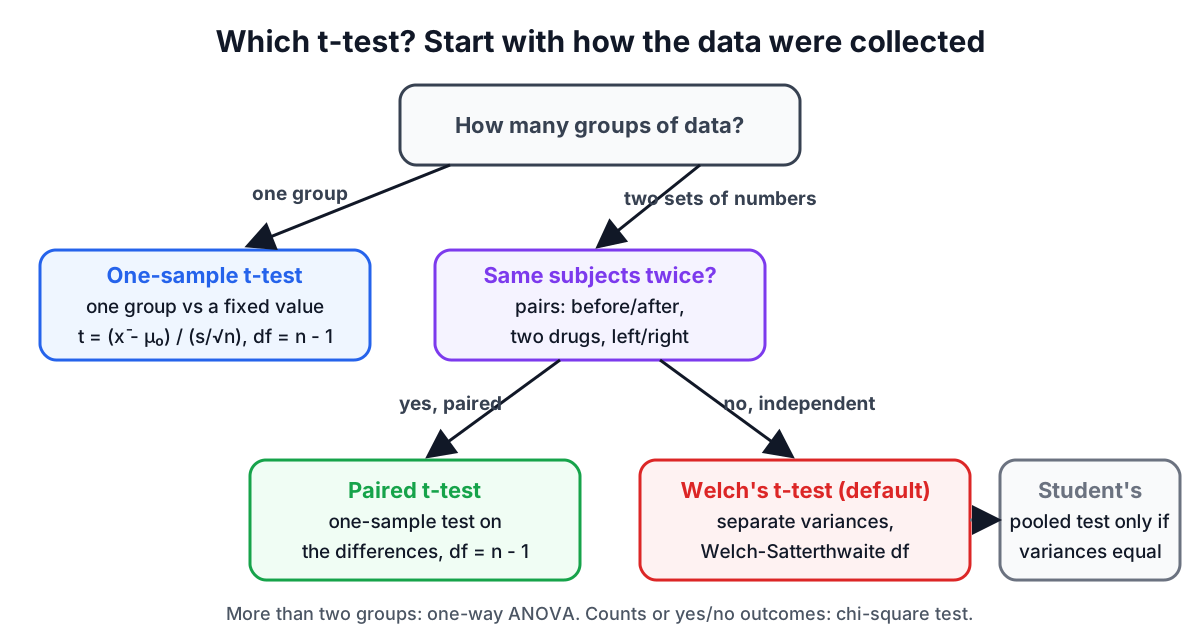
- One group against a fixed number? A one-sample t-test. Example: is the mean fill weight of a production run different from the 500 g label?
- Two measurements on the same subjects? A paired t-test. Examples: blood pressure before and after treatment, two drugs given to the same patients, left and right eye.
- Two separate groups of subjects? A two-sample t-test. Examples: a control and a treatment group, two classes, two website variants.
- For two separate groups, are the variances equal? You rarely know. Use Welch's test unless there is a strong reason to assume equal variances.
The one-sample t-test
The statistic is
t = (x̄ - μ₀) / (s / √n), with n - 1 degrees of freedom.
The denominator s / √n is the standard error of the mean. Suppose 12 bags have a mean of 497.8 g and a standard deviation of 3.1 g, tested against the 500 g label. The standard error is 3.1 / √12 = 0.895, so t = (497.8 - 500) / 0.895 = -2.46 with 11 degrees of freedom. The two-sided p-value is about 0.032. The 95% confidence interval for the mean is 497.8 ± 2.201 × 0.895, or 495.8 to 499.8 g, which excludes 500, matching the significant result.
The paired t-test: Student's own data
A paired test is a one-sample test on the differences. Student illustrated his 1908 paper with sleep data from Cushny and Peebles (1905): the extra hours of sleep ten patients got from two different drugs. The same data ship with R as the sleep data set.
| Patient | 1 | 2 | 3 | 4 | 5 | 6 | 7 | 8 | 9 | 10 |
|---|---|---|---|---|---|---|---|---|---|---|
| Drug 1 | 0.7 | -1.6 | -0.2 | -1.2 | -0.1 | 3.4 | 3.7 | 0.8 | 0.0 | 2.0 |
| Drug 2 | 1.9 | 0.8 | 1.1 | 0.1 | -0.1 | 4.4 | 5.5 | 1.6 | 4.6 | 3.4 |
| Difference | -1.2 | -2.4 | -1.3 | -1.3 | 0.0 | -1.0 | -1.8 | -0.8 | -4.6 | -1.4 |
The differences have mean -1.58 and standard deviation 1.230. The standard error is 1.230 / √10 = 0.389, so t = -1.58 / 0.389 = -4.062 with 9 degrees of freedom, and the two-sided p-value is 0.0028. The 95% interval for the mean difference is -1.58 ± 2.262 × 0.389, or -2.46 to -0.70 hours. These match R's t.test(x, y, paired = TRUE) exactly.
What pairing buys
Now treat the same two columns as if they came from twenty different people. Welch's two-sample test gives t = -1.861 with 17.8 degrees of freedom and p = 0.079: not significant. The difference in means is identical, -1.58 hours. What changed is the error term. Patients differ a lot from each other (patient 9 gained 4.6 hours on drug 2, patient 5 gained nothing on either), and an independent-groups test has to include all that person-to-person spread. Pairing subtracts it out, because each patient is compared with themselves.
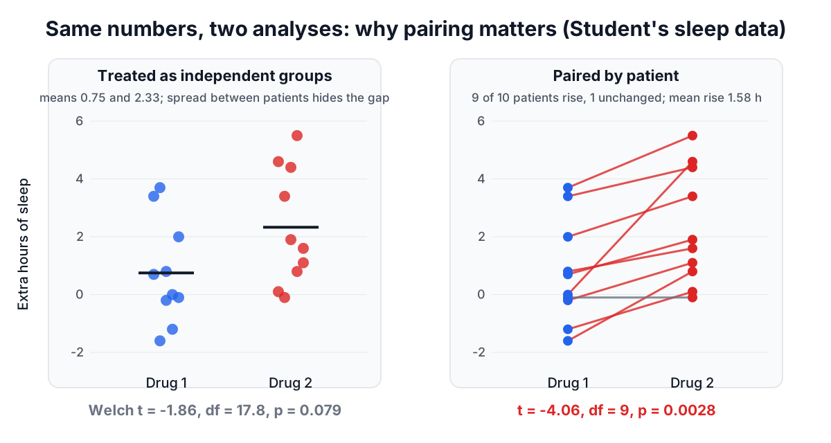
The lesson runs both ways. If your data are paired, analyse them as paired or you throw away power. If they are not paired, a paired test is simply wrong; you cannot pair the third person in group A with the third person in group B because they happen to be in the same row.
Two independent groups: Student or Welch?
Student's pooled test assumes both groups share one variance. It averages the two sample variances, weighted by degrees of freedom:
- s_p² = ((n₁ - 1)s₁² + (n₂ - 1)s₂²) / (n₁ + n₂ - 2)
- SE = s_p · √(1/n₁ + 1/n₂), with n₁ + n₂ - 2 degrees of freedom
Welch's test, published by Bernard Welch in 1947, keeps the variances separate:
- SE = √(s₁²/n₁ + s₂²/n₂)
- df = (s₁²/n₁ + s₂²/n₂)² / [ (s₁²/n₁)² / (n₁ - 1) + (s₂²/n₂)² / (n₂ - 1) ]
The degrees of freedom formula is the Welch-Satterthwaite approximation, and it usually gives a fractional answer between the smaller group's n - 1 and n₁ + n₂ - 2.
When the variances really are equal, both tests give nearly the same answer. When they differ, and especially when the smaller group has the larger variance, the pooled test's false-positive rate can drift well above the nominal 5%. Welch's test stays close to it. Testing for equal variances first and then choosing does not fix the problem, because the preliminary test has low power exactly when it matters. That is why R's t.test defaults to Welch, and why the calculator does too.
A worked example from summary statistics
Two classes sit the same test. Class A: mean 24.6, SD 4.2, n = 18. Class B: mean 21.3, SD 5.1, n = 20.
- s₁²/n₁ = 17.64 / 18 = 0.980 and s₂²/n₂ = 26.01 / 20 = 1.3005
- SE = √(0.980 + 1.3005) = 1.510
- t = (24.6 - 21.3) / 1.510 = 2.185
- df = 2.2805² / (0.980² / 17 + 1.3005² / 19) = 35.74
- two-sided p = 0.0355, and the 95% CI for the difference is 0.24 to 6.36 points
The pooled test gives t = 2.163 with 36 df and p = 0.0373. Close, because the variances are not very different.
Reading the result
A t-test produces several numbers, and the p-value is the least informative on its own.
The p-value is the probability of a t statistic at least as extreme as yours if the true difference were the hypothesised value (usually zero). It is not the probability that the null hypothesis is true. See the p-value guide for the common misreadings.
The confidence interval gives the range of differences compatible with the data. An interval of 0.24 to 6.36 says the true advantage of class A could be tiny or substantial; that is more useful than "p = 0.036".
One-sided tests halve the p-value when the effect is in the predicted direction. Use one only if the direction was fixed before you collected the data and an effect in the other direction would be treated the same as no effect. Choosing the tail after looking doubles your real false-positive rate.
Effect size: Cohen's d
Statistical significance depends on sample size; a trivial difference becomes significant with enough data. Cohen's d expresses the difference in standard deviation units:
- two independent groups: d = (x̄₁ - x̄₂) / s_p
- paired data: d = mean difference / SD of the differences (sometimes written d_z)
For the two classes, s_p = 4.70, so d = 3.3 / 4.70 = 0.70. Jacob Cohen suggested 0.2, 0.5 and 0.8 as rough markers of small, medium and large effects, while warning that they are a fallback when a field has no better benchmark. Hedges' g multiplies d by 1 - 3 / (4(n₁ + n₂) - 9) to remove a small upward bias in small samples; here g = 0.69.
Assumptions and when to use something else
- Independence. Observations within each group must be independent. Clustered data (pupils within schools, repeated readings from one machine) need a multilevel model.
- Approximate normality of the mean. With small samples the data themselves should be roughly symmetric without extreme outliers. With about 30 or more per group, the central limit theorem usually makes the mean close enough to normal. For small, skewed samples, the Wilcoxon signed-rank test (paired) or the Mann-Whitney U test (independent) are common alternatives.
- More than two groups. Running every pairwise t-test inflates the false-positive rate. Use a one-way ANOVA first.
- Proportions, not means. For yes/no outcomes such as conversion rates, a test on counts like the chi-square test fits better.
How to report a t-test
A complete report names the test, gives the means and standard deviations, the statistic with its degrees of freedom, the exact p-value, the confidence interval and an effect size. For example:
Class A scored higher than class B (M = 24.6, SD = 4.2, n = 18 vs M = 21.3, SD = 5.1, n = 20), Welch's t(35.7) = 2.19, p = 0.036, mean difference 3.3, 95% CI [0.24, 6.36], d = 0.70.
The calculator's Copy result button produces the numbers in this order.
Sources
- Student (1908). The probable error of a mean. Biometrika, 6(1), 1-25.
- Cushny, A. R. and Peebles, A. R. (1905). The action of optical isomers II: hyoscines. Journal of Physiology, 32, 501-510.
- Welch, B. L. (1947). The generalization of "Student's" problem when several different population variances are involved. Biometrika, 34, 28-35.
- Satterthwaite, F. E. (1946). An approximate distribution of estimates of variance components. Biometrics Bulletin, 2(6), 110-114.
- Cohen, J. (1988). Statistical Power Analysis for the Behavioral Sciences, 2nd ed.
- R Core Team,
t.testandsleepdocumentation.
Related searches
- how to do a t test
- paired vs independent t test
- welch vs student t test
- welch satterthwaite formula
- t test degrees of freedom
- cohens d interpretation
- student 1908 guinness
- one tailed or two tailed t test