
One-Way ANOVA Explained: F, Effect Sizes and Post Hoc Tests
Splitting variation into between and within groups, building the ANOVA table, why F works, Welch's ANOVA for unequal variances, eta and omega squared, and Holm-adjusted comparisons.
· 11 min read

One-way analysis of variance (ANOVA) compares the means of three or more groups in a single test. Despite the name, it is a test about means; it gets there by comparing two estimates of variance. This guide builds an ANOVA table by hand from a small published data set, explains why the F ratio works, covers effect sizes, Welch's ANOVA for unequal variances and how to find which groups differ, and lists the assumptions to check. The One-Way ANOVA Calculator produces every number shown here.
Why not several t-tests?
With three groups you could run three t-tests: A against B, A against C, B against C. The trouble is that each test carries its own 5% chance of a false positive when there is no real difference. With independent tests, the chance of at least one false alarm across k tests is 1 - 0.95^k:
| Groups | Pairs | Chance of at least one false positive |
|---|---|---|
| 3 | 3 | 14% |
| 4 | 6 | 26% |
| 5 | 10 | 40% |
| 7 | 21 | 66% |
(The pairwise tests share data, so the real figures are a little lower, but the problem is the same.) ANOVA asks one question, "are all the means equal?", at one error rate.
The idea: two estimates of the same variance
Ronald Fisher developed analysis of variance at the Rothamsted Experimental Station in the 1920s to analyse crop trials and published it in Statistical Methods for Research Workers (1925). The logic runs like this.
- The scatter of values within each group estimates the error variance, whatever the group means are.
- The scatter of the group means between groups also estimates the error variance, but only if the true means are equal. If they differ, the between-group scatter is inflated by the real differences.
So compute both and take their ratio. Under the null hypothesis the ratio, F, should be near 1. Large values of F mean the group means are further apart than the within-group noise can explain. George Snedecor named the F distribution after Fisher in 1934.
A worked example: PlantGrowth
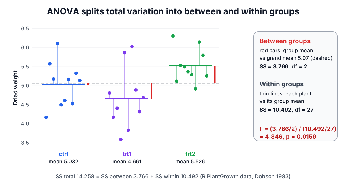
The PlantGrowth data, from Annette Dobson's An Introduction to Statistical Modelling (1983) and shipped with R, record the dried weight of 30 plants: 10 controls and 10 under each of two treatments.
| Group | n | Mean | SD |
|---|---|---|---|
| ctrl | 10 | 5.032 | 0.5831 |
| trt1 | 10 | 4.661 | 0.7937 |
| trt2 | 10 | 5.526 | 0.4426 |
The grand mean of all 30 plants is 5.073.
Step 1: sum of squares between groups
SS_between = Σ nᵢ (x̄ᵢ - grand mean)² = 10 × (5.032 - 5.073)² + 10 × (4.661 - 5.073)² + 10 × (5.526 - 5.073)² = 0.0168 + 1.6974 + 2.0521 = 3.7663
Step 2: sum of squares within groups
SS_within = Σ (nᵢ - 1) sᵢ² = 9 × 0.5831² + 9 × 0.7937² + 9 × 0.4426² = 3.0601 + 5.6694 + 1.7628 = 10.4921
The two add up to the total sum of squares around the grand mean, 14.2584. That identity, SS_total = SS_between + SS_within, is the "analysis" of variance.
Step 3: degrees of freedom and mean squares
With k = 3 groups and N = 30 plants, df_between = k - 1 = 2 and df_within = N - k = 27. Dividing each sum of squares by its degrees of freedom gives the mean squares:
- MS_between = 3.7663 / 2 = 1.8832
- MS_within = 10.4921 / 27 = 0.3886
Step 4: F and p
F = 1.8832 / 0.3886 = 4.846. The right-tail area of an F distribution with 2 and 27 degrees of freedom beyond 4.846 is p = 0.0159. The full table:
| Source | SS | df | MS | F | p |
|---|---|---|---|---|---|
| Between groups | 3.766 | 2 | 1.883 | 4.846 | 0.0159 |
| Within groups | 10.492 | 27 | 0.389 | ||
| Total | 14.258 | 29 |
This matches R's summary(aov(weight ~ group, data = PlantGrowth)). At α = 0.05 we reject the hypothesis that all three means are equal.
Because the table needs only n, mean and SD per group, you can run an ANOVA from the summary statistics in a published paper. The calculator's "n, mean, SD" mode does exactly that.
How big is the effect?
Eta squared is the share of total variation that lies between groups: η² = SS_between / SS_total = 3.766 / 14.258 = 0.264. About a quarter of the variation in weight goes with the group.
η² describes this sample and is biased upwards as an estimate of the population effect, especially with small groups. Omega squared corrects for that:
ω² = (SS_between - df_between × MS_within) / (SS_total + MS_within) = (3.766 - 2 × 0.3886) / (14.258 + 0.3886) = 0.204
Report ω² when you want an estimate of the effect in the population.
Which groups differ? Post hoc comparisons
A significant F says that not all means are equal. It does not say which ones differ. The usual next step compares every pair, with an adjustment for the number of comparisons.
The calculator uses t-tests on the pooled within-group variance: for groups i and j, t = (x̄ᵢ - x̄ⱼ) / √(MS_within × (1/nᵢ + 1/nⱼ)) with N - k degrees of freedom. Each raw p-value is then adjusted two ways:
- Bonferroni multiplies each p-value by the number of comparisons (capped at 1). Simple and conservative.
- Holm (1979) sorts the p-values, multiplies the smallest by m, the next by m - 1 and so on, keeping the sequence non-decreasing. It controls the same overall error rate and is never less powerful than Bonferroni, so there is little reason to prefer Bonferroni.
For PlantGrowth:
| Pair | Difference | t | Raw p | Holm | Bonferroni |
|---|---|---|---|---|---|
| ctrl vs trt1 | 0.371 | 1.331 | 0.194 | 0.194 | 0.583 |
| ctrl vs trt2 | -0.494 | -1.772 | 0.088 | 0.175 | 0.263 |
| trt1 vs trt2 | -0.865 | -3.103 | 0.0045 | 0.0134 | 0.0134 |
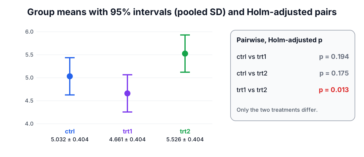
Only the two treatments differ from each other; neither differs clearly from the control. The overall effect comes from the treatments pulling in opposite directions. These values match R's pairwise.t.test(weight, group) with Holm (its default) and Bonferroni adjustments. Tukey's honestly significant difference (HSD) test is a common alternative designed for all pairwise comparisons; it uses the studentized range distribution and gives similar conclusions here, but this calculator does not compute it.
Unequal variances: Welch's ANOVA
The classic F test assumes every group has the same variance. With equal group sizes it tolerates moderate differences, but when variances and group sizes both differ, and especially when the smallest group has the largest variance, its false-positive rate can drift far from α.
Bernard Welch proposed a fix in 1951. Each group gets a weight wᵢ = nᵢ / sᵢ², the group means are compared around a weighted grand mean, and the denominator degrees of freedom are estimated from the data, much like Welch's t-test. For PlantGrowth, Welch's F = 5.181 with 2 and 17.13 degrees of freedom, p = 0.0174, the same conclusion as the classic test. In R this is oneway.test(weight ~ group, data = PlantGrowth).
To check the assumption, Levene's test runs an ANOVA on the absolute deviations of each value from its group centre. The version using the group median, due to Brown and Forsythe (1974), is less sensitive to non-normal data and is the default in R's car::leveneTest and SciPy's levene. For PlantGrowth it gives F(2, 27) = 1.119, p = 0.341: no strong sign of unequal variances. Many statisticians skip the preliminary test and simply report Welch's ANOVA whenever group spreads look different, since it loses little when variances are equal.
Assumptions checklist
- Independent observations. Each value comes from a different, unrelated subject. Measuring the same subjects under several conditions needs repeated-measures ANOVA or a mixed model.
- Approximately normal residuals within groups. ANOVA is fairly tolerant of mild non-normality, especially with balanced groups of 15 or more. For small, skewed groups the Kruskal-Wallis test is a rank-based alternative.
- Equal variances. Check the SDs (a ratio of largest to smallest above about 2 is a warning sign) and Levene's test, or use Welch's ANOVA.
Connections
With exactly two groups, one-way ANOVA and the pooled two-sample t-test are the same test: F = t² and the p-values match. ANOVA is also a special case of linear regression with the group coded as indicator variables, which is why the ANOVA table in regression output looks the same. For what the p-value in the table does and does not mean, see the p-value guide.
Reporting an ANOVA
Give the F statistic with both degrees of freedom, the p-value, an effect size, and the follow-up comparisons:
Plant weight differed between groups, F(2, 27) = 4.85, p = 0.016, ω² = 0.20. Holm-adjusted comparisons showed that trt2 plants were heavier than trt1 plants (difference 0.87, p = 0.013); neither treatment differed from the control.
Sources
- Fisher, R. A. (1925). Statistical Methods for Research Workers. Oliver and Boyd.
- Dobson, A. J. (1983). An Introduction to Statistical Modelling. Chapman and Hall.
- Welch, B. L. (1951). On the comparison of several mean values: an alternative approach. Biometrika, 38, 330-336.
- Levene, H. (1960). In I. Olkin (ed.), Contributions to Probability and Statistics: Essays in Honor of Harold Hotelling, 278-292. Stanford University Press.
- Brown, M. B. and Forsythe, A. B. (1974). Journal of the American Statistical Association, 69(346), 364-367 (the median-centred variance test).
- Holm, S. (1979). A simple sequentially rejective multiple test procedure. Scandinavian Journal of Statistics, 6, 65-70.
Related searches
- one way anova explained
- anova table example
- how to calculate f statistic
- welch anova vs classic anova
- post hoc test after anova
- eta squared vs omega squared
- multiple comparisons problem
- anova assumptions levene test