
LMTD and the F Correction Factor: Sizing Heat Exchangers
Where the log mean temperature difference comes from, why counterflow beats parallel flow, how the shell-and-tube F factor is calculated and when F gets too low to trust.
· 10 min read

Every heat exchanger calculation eventually reaches the same equation: duty equals overall heat transfer coefficient times area times a temperature difference. The trouble is that the temperature difference between the two fluids changes along the length of the exchanger, sometimes by a factor of five or more. The log mean temperature difference (LMTD) is the correct average to use, and the F correction factor adapts it to real multi-pass exchangers. This post derives both, with the numbers from the LMTD Calculator.
Why an average is needed
Consider a small slice of exchanger area dA. Heat crosses it at a rate set by the local difference between hot and cold fluid temperatures:
dQ = U x (Th − Tc) x dA
As the fluids move along, the hot one cools and the cold one warms, so Th − Tc changes from one end to the other. To get the total duty you have to integrate. Assume U is constant, the specific heats are constant, there is no phase change and no heat loss to the surroundings. Then each stream's temperature changes in proportion to the heat it has exchanged, and the difference ΔT = Th − Tc changes linearly with Q. Writing dQ = U·ΔT·dA and integrating from one end (ΔT1) to the other (ΔT2) gives
Q = U x A x (ΔT1 − ΔT2) / ln(ΔT1 / ΔT2)
The fraction is the log mean temperature difference. It is always smaller than the arithmetic mean, and the gap widens as the two end differences move apart. With ΔT1 = 80 K and ΔT2 = 60 K the LMTD is 69.52 K against an arithmetic mean of 70 K, a small difference. With 120 K and 20 K the LMTD is 55.8 K against 70 K, and using the arithmetic mean would overstate the duty by 25%.
When ΔT1 equals ΔT2 the formula becomes 0/0. The limit is simply the common value, which makes sense: if the difference is the same at both ends of a linear profile, it is the same everywhere. This happens in a counterflow exchanger where both streams have the same heat capacity rate (mass flow times specific heat). The calculator detects it and returns ΔT1 directly instead of dividing by zero.
Counterflow versus parallel flow
The two end differences depend on how the streams are arranged.
Counterflow:    ΔT1 = Th,in − Tc,out     ΔT2 = Th,out − Tc,in
Parallel flow:  ΔT1 = Th,in − Tc,in      ΔT2 = Th,out − Tc,out
Take the calculator's default: hot water from 150 °C to 90 °C, cold water from 30 °C to 70 °C.
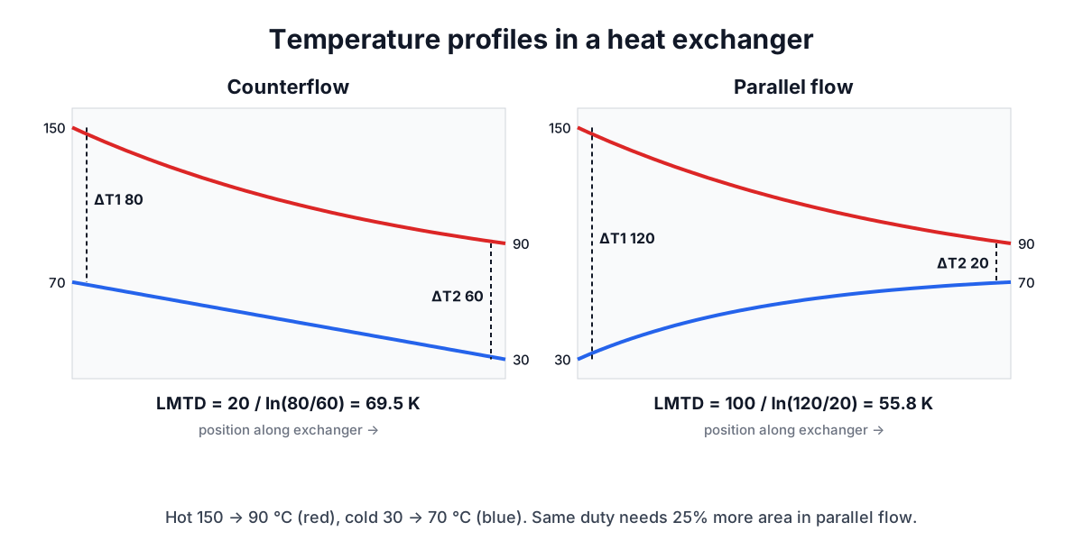
In counterflow the gap stays fairly even along the length, between 80 K and 60 K. In parallel flow it starts at 120 K and collapses to 20 K at the outlet, so much of the exchanger works with very little driving force. For U = 500 W/m²·K and 10 m², counterflow delivers 500 x 10 x 69.52 = 347.6 kW. Parallel flow needs 347,600 / (500 x 55.81) = 12.46 m² for the same duty, about 25% more area.
Counterflow has a second advantage. Its cold outlet can be hotter than the hot outlet, a temperature cross. In parallel flow both outlets approach the same temperature and the cold outlet can never exceed the hot outlet. If you enter a parallel-flow case where it would, the calculator reports that both end differences must be positive.
The F correction factor
Most shell-and-tube exchangers are not pure counterflow. In the common 1-2 arrangement, the shell fluid makes one pass while the tube fluid goes down and back, so half of the tube length runs counter to the shell flow and half runs parallel to it. The effective temperature difference falls between the two pure cases. It is written as the counterflow LMTD multiplied by a correction factor F of 1 or less:
Q = U x A x F x LMTD_counterflow
F depends on two dimensionless ratios:
R = (Th,in − Th,out) / (Tc,out − Tc,in)     ratio of temperature changes
P = (Tc,out − Tc,in) / (Th,in − Tc,in)      cold-side effectiveness
For one shell pass and any even number of tube passes, Bowman, Mueller and Nagle (1940) gave a closed form, reproduced in the TEMA standards and heat transfer textbooks:
F = [√(R²+1) / (R−1)] x ln[(1−P)/(1−PR)]
    / ln[(2 − P(R+1−√(R²+1))) / (2 − P(R+1+√(R²+1)))]
with a separate limit for R = 1. For the default temperatures R = 60/40 = 1.5 and P = 40/120 = 0.333, giving F = 0.910. The area for 347.6 kW becomes 347,600 / (500 x 0.910 x 69.52) = 10.98 m².
F has a useful symmetry: F(R, P) = F(1/R, PR), which means it does not matter which fluid goes in the shell as far as F is concerned. The calculator's test suite checks this property.
How low can F go
F falls as the outlet temperatures approach each other and drops off a cliff near the limit of what a single shell can achieve. For R = 1 the curve hits zero at P ≈ 0.586; beyond that the 1-2 exchanger cannot do the duty at all, and the calculator reports "no solution". Long before that point, F becomes so sensitive that a 1 K error in a predicted temperature can change the required area by tens of percent.
Common practice is to keep F above about 0.8 and never design below 0.75. When F gets too low the options are:
- two or more shells in series, which approaches true counterflow (charts exist for 2-4, 3-6 and so on);
- a different exchanger type, such as a plate exchanger, which is close to pure counterflow;
- relaxing the temperature approach if the process allows it.
When one stream is condensing or boiling at constant temperature, R or P is zero and F is exactly 1 for any arrangement, so the counterflow LMTD can be used directly.
Using LMTD in practice
- Balance the duty first. The hot side's m·cp·ΔT must equal the cold side's. If you only know three temperatures, compute the fourth from the heat balance before using the LMTD.
- Use a design U with fouling. Clean overall coefficients can drop 20 to 50% after scale and biological growth build up. TEMA lists fouling resistances by fluid.
- Split variable-property cases into zones. A condenser that also subcools, or a fluid whose specific heat changes strongly, breaks the linear assumption. Calculate each zone with its own LMTD and U.
- Check against the NTU method. For rating an existing exchanger, where outlet temperatures are unknown, the effectiveness-NTU method avoids iteration. Both methods give the same answer for the same exchanger.
For the energy each stream carries, the Specific Heat Calculator handles Q = m·c·ΔT, and the post on specific and latent heat covers phase change duty. The flow side is covered by the Flow Rate Calculator, the Reynolds Number Calculator for whether the tube flow is turbulent, and the Pipe Pressure Drop Calculator for the pumping cost of a design.