
Normal Distribution Probabilities and the Inverse Normal
Standardising with z, finding areas below, above and between values, the 68-95-99.7 rule, working backwards to percentiles, and when the bell curve is the wrong model.
· 10 min read

The normal distribution is the bell curve behind exam percentiles, manufacturing tolerances, reference ranges and most of the critical values in statistics. Two kinds of question come up again and again: given a value, what share of the distribution lies below, above or between values; and given a share, which value cuts it off. This guide shows how to answer both by standardising to z, works through the common question types, explains the 68-95-99.7 rule, and spells out when the bell curve is the wrong tool. The Normal Distribution Calculator does every calculation here in your own units and shades the area.
Where the bell curve comes from
Abraham de Moivre found the curve in 1733 while approximating the probabilities of many coin tosses. Pierre-Simon Laplace and Carl Friedrich Gauss developed it around 1809 and 1810 as the law of errors in astronomical measurements, which is why it is also called the Gaussian distribution. Laplace's central limit theorem explains why it turns up so often: the sum or average of many small, independent effects tends towards a normal shape, whatever the shape of the individual effects.
A normal distribution is fixed by two numbers, the mean μ (its centre) and the standard deviation σ (its spread). The curve is symmetric about μ, its inflection points are at μ ± σ, and its tails never quite reach zero. The density is
f(x) = (1 / (σ√(2π))) × exp(-(x - μ)² / (2σ²))
and probabilities are areas under this curve. The total area is 1.
Standardising: every normal is one curve
Any normal distribution can be turned into the standard normal (mean 0, standard deviation 1) by measuring distance from the mean in standard deviations:
z = (x - μ) / σ
The probability below x is then Φ(z), the area to the left of z under the standard curve. Φ has no closed-form expression, which is why textbooks print z-tables to four decimal places. Software evaluates it with series and continued fractions to full double precision; the calculator uses George Marsaglia's 2004 series in the centre and a continued fraction in the tails, so even P(Z > 8) = 6.2 × 10⁻¹⁶ comes out correctly rather than as zero.
Four probability questions
All examples use the IQ scale, which is designed to have mean 100 and standard deviation 15.
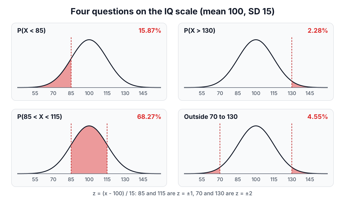
Below a value. P(X < 85): z = (85 - 100) / 15 = -1, and Φ(-1) = 0.15866. About 15.9% of people score below 85.
Above a value. P(X > 130): z = 2, and the right tail is 1 - Φ(2) = 0.02275, about 1 person in 44. Computing the upper tail directly instead of subtracting from 1 matters only far out in the tail, but there it matters a lot: 1 - 0.9999999999 loses most of its digits in floating point.
Between two values. P(85 < X < 115) = Φ(1) - Φ(-1) = 0.84134 - 0.15866 = 0.68269.
Outside two values. P(X < 70 or X > 130) = Φ(-2) + (1 - Φ(2)) = 0.04550. This is the form of a two-sided specification check: what fraction of parts falls outside the tolerance band?
For a continuous distribution the probability of hitting an exact value is zero, so "<" and "≤" give the same answer.
The 68-95-99.7 rule
Three areas are worth knowing by heart:
| Range | Share inside | Share outside |
|---|---|---|
| μ ± 1σ | 68.27% | 31.73% |
| μ ± 2σ | 95.45% | 4.55% |
| μ ± 3σ | 99.73% | 0.27% |
| μ ± 1.96σ | 95.00% | 5.00% |
| μ ± 2.576σ | 99.00% | 1.00% |
The last two rows are where the 1.96 and 2.576 multipliers in 95% and 99% confidence intervals come from. The rule is a quick check on any normal calculation: if you get 40% between μ - σ and μ + σ, something has gone wrong.
Working backwards: the inverse normal
The inverse question starts from a probability. Which score marks the 90th percentile? Which value has only 5% of the distribution above it? This is the inverse normal, Φ⁻¹, also called the quantile function, Excel's NORM.INV and the TI-84's invNorm.
The steps reverse the standardisation:
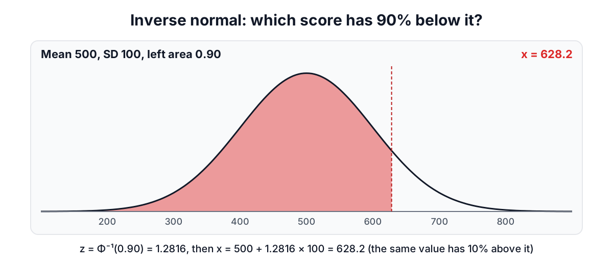
- Find z with the required area. For the 90th percentile, z = Φ⁻¹(0.90) = 1.28155.
- Convert back: x = μ + z × σ.
With a test scored with mean 500 and standard deviation 100, the 90th percentile is 500 + 1.28155 × 100 = 628.2. The same value has 10% above it, so "right-tail area 0.1" gives the same answer.
Symmetric limits work the same way. The middle 95% of IQ scores lies between 100 - 1.95996 × 15 = 70.60 and 100 + 1.95996 × 15 = 129.40. "Central 95%" and "5% in the two tails" are the same question asked from opposite sides.
The calculator computes Φ⁻¹ with Peter Acklam's rational approximation, accurate to about 1 part in 10⁹, followed by one Halley correction step against the accurate Φ, which brings it to full double precision.
Practical uses
Exam grading. If marks are roughly normal with mean 62 and SD 11, the share above a pass mark of 50 is P(Z > -1.09) = 86%. The mark needed for the top 10% is 62 + 1.28155 × 11 = 76.1.
Manufacturing tolerances. A shaft is specified at 25.00 ± 0.05 mm and the process runs at mean 25.01 mm with SD 0.02 mm. The share out of tolerance is P(X < 24.95) + P(X > 25.05) = Φ(-3) + (1 - Φ(2)) = 0.00135 + 0.02275 = 2.4%. Centring the process at 25.00 would cut that to 2 × Φ(-2.5) = 1.24%. This is the arithmetic behind process capability indices.
Reference ranges. Many lab reference ranges are set as the central 95% of a healthy population, mean ± 1.96 SD. By construction, 1 healthy person in 20 falls outside the range, which is why a single slightly abnormal result is not alarming on its own.
Normal approximations to counts
A binomial count with n trials and probability p has mean np and standard deviation √(np(1 - p)). When np and n(1 - p) are both at least about 10, the normal curve approximates it well, which is de Moivre's original result. Because counts are whole numbers, a continuity correction improves the approximation: P(X ≤ 45) becomes P(X < 45.5) on the normal curve. For 100 tosses of a fair coin, P(at most 45 heads) is about Φ((45.5 - 50) / 5) = Φ(-0.9) = 0.184; the exact binomial value is 0.184 as well.
When not to use the normal curve
The normal model is a good description of many things and a bad description of many others.
- Skewed data. Incomes, house prices, insurance claims, reaction times and waiting times have long right tails. A normal model badly underestimates the chance of large values and may even give positive probability to impossible negative ones.
- Heavy tails. Daily stock returns have far more extreme days than a normal curve allows. Under a normal model, a daily move of 5 standard deviations in either direction should come about once in 7,000 years of trading; markets have produced many within living memory.
- Bounded or discrete data. Ratings on a 1 to 5 scale, counts near zero and percentages near 0% or 100% are poorly served by a symmetric curve.
- Small samples from an unknown distribution. With a handful of observations you cannot tell whether the data are normal. For a mean whose standard deviation is estimated from the same small sample, use the t distribution instead (see the t-test guide).
Before relying on tail probabilities, plot the data. A histogram or a normal quantile plot shows quickly whether the bell curve fits. Sample means are a different matter: by the central limit theorem they are often close to normal even when individual values are not, which is why the normal curve underlies so many tests. For converting test statistics to p-values with the normal and related distributions, see the p-value guide.
Sources
- de Moivre, A. (1733). Approximatio ad summam terminorum binomii (a + b)ⁿ in seriem expansi.
- Gauss, C. F. (1809). Theoria motus corporum coelestium.
- Marsaglia, G. (2004). Evaluating the normal distribution. Journal of Statistical Software, 11(4).
- Acklam, P. J. An algorithm for computing the inverse normal cumulative distribution function (web publication).
- NIST/SEMATECH e-Handbook of Statistical Methods, section 1.3.6.6.1, Normal distribution.
Related searches
- normal distribution probability
- area under the normal curve
- inverse normal percentile
- empirical rule 68 95 99.7
- how to standardise a normal variable
- normal approximation continuity correction
- process capability out of spec
- central limit theorem explained