
Time Value of Money: PV, FV, NPV, IRR, CAGR and ROI Explained
One growth factor behind present value, future value, NPV, IRR, CAGR and ROI: how each is calculated, when each misleads, and which to use for a decision.
· 9 min read

Would you rather have 1,000 today or 1,000 in five years? Everyone picks today, and not only out of impatience. Money you hold now can be invested, so a dollar today is worth more than a dollar later. Turning that intuition into numbers is called the time value of money, and it sits underneath present value, future value, net present value, internal rate of return, CAGR and annualized ROI.
This guide works through each of those measures with real numbers from the Present and Future Value Calculator, the NPV and IRR Calculator, the CAGR Calculator and the ROI Calculator. The aim is to show where each one comes from, what question it answers, and where it quietly gives a wrong impression. It explains the maths; it is not advice on any particular investment.
One growth factor behind everything
Every calculation here is built from a single expression, (1 + i)^n, where i is the interest rate per period and n is the number of periods. Multiply by it and money moves forward in time. Divide by it and money moves back.
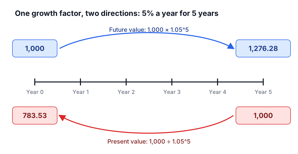
At 5% a year for five years the factor is 1.05^5 = 1.27628. So 1,000 invested today becomes 1,276.28, which is its future value. And 1,000 promised in five years is worth 1,000 ÷ 1.27628 = 783.53 today, which is its present value. The two are the same statement read in opposite directions: if you could earn 5% elsewhere, 783.53 now and 1,000 in five years are equally good.
The rate you divide by is called the discount rate. It should be the return you could get on something of similar risk, which is why the same future payment is worth more to a person whose alternative is a 3% savings account than to one whose alternative is a 10% business.
Payment streams and the annuity formulas
Most real problems involve a series of equal payments: rent, loan repayments, pension income, monthly savings. You could discount each payment separately and add them, but the sum collapses into two compact formulas:
FV of payments = PMT × [((1 + i)^n − 1) ÷ i]
PV of payments = PMT × [(1 − (1 + i)^−n) ÷ i]
These assume each payment arrives at the end of its period, an ordinary annuity. If payments arrive at the start, an annuity due, every payment gets one extra period, so both formulas are multiplied by (1 + i). With 1,000 a year for ten years at 5%, the present value is 7,721.73 as an ordinary annuity and 8,107.82 as an annuity due. Those are the values in every printed annuity table, and the calculator reproduces them.
Two practical details trip people up. First, the rate must match the payment period. A nominal 6% compounded monthly is 0.5% per month, and if payments are yearly but compounding is quarterly, the per-payment rate is (1 + 0.06/4)^4 − 1. The Present and Future Value Calculator converts this automatically and shows the rate it used. Second, a stream that never ends (a perpetuity) has a finite present value: payment ÷ rate. At 5%, 1,000 a year forever is worth 20,000 today, which is why very long annuities barely gain value as you add years.
For more on how compounding frequency changes the effective rate, see the compound interest guide.
Net present value: is the project worth more than it costs?
A project usually costs money up front and returns uneven amounts later. Net present value discounts each flow to today and adds them, with the initial outlay at period 0 left undiscounted:
NPV = CF0 + CF1 ÷ (1 + r) + CF2 ÷ (1 + r)^2 + ... + CFn ÷ (1 + r)^n
Take a project costing 50,000 that returns 12,000, 15,000, 18,000, 20,000 and 9,000 over five years. At an 8% discount rate the NPV is 9,086.02. That number has a precise meaning: after paying back the 50,000 and earning 8% on it along the way, the project leaves 9,086 of extra value in present-day money. Positive NPV means accept, negative means reject, at that rate.
One warning for spreadsheet users: the NPV() function in Excel and Google Sheets discounts the first value you give it by a full period. If you include the period 0 investment inside it, the result is wrong by a factor of (1 + r). Write =NPV(8%, B2:B6) + B1 instead.
IRR, and why it sometimes has two answers
The internal rate of return is the discount rate at which NPV is exactly zero. Plot NPV against the rate, the NPV profile, and the IRR is where the curve crosses the axis.
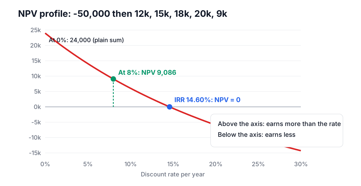
For the project above the IRR is 14.60%. Since 14.60% is above the 8% hurdle, IRR and NPV agree. They usually do for a conventional project: one outflow followed by inflows gives one sign change and exactly one IRR.
Things change when the cash flows switch sign more than once. A mine or a power plant costs money to build, earns for years, then costs money again to close. Consider -100, then +230, then -132. NPV is zero at both 10% and 20%, positive between them and negative outside. Both are genuine IRRs, and a spreadsheet IRR() returns whichever one its starting guess happens to reach. Descartes' rule of signs puts the ceiling: the number of IRRs can be no more than the number of sign changes.
Some flows have no IRR at all. A project costing 1,000,000, earning 300,000 for four years and then costing 400,000 to dismantle has a negative NPV at every rate, so there is nothing to find. A solver that only runs Newton's method from a guess may stop with an error or return nonsense. The NPV and IRR Calculator scans NPV across rates from -99% to 10,000%, finds every interval where it changes sign, and refines each crossing with Newton steps that fall back to bisection when a step would escape the interval. It then reports every IRR, or says plainly that there is none.
MIRR and payback: the supporting cast
MIRR (modified IRR) avoids both problems. Outflows are discounted to today at a finance rate, inflows are compounded to the final year at a reinvestment rate, and MIRR is the single rate that links the two totals. For the 50,000 project with both rates at 8%, MIRR is 11.67%, lower than the 14.60% IRR. The gap reflects an assumption hidden inside IRR: that every cash flow received can be reinvested at the IRR itself. If your realistic reinvestment rate is 8%, MIRR is the better description of what the project earns. For the closing-cost example with no IRR, MIRR at 10% is still a usable 4.17%.
Payback period is how long until the cumulative cash flow turns positive. The 50,000 project gets its money back after 3.25 years. Discounted payback does the same with present values and takes 3.80 years. Payback is a liquidity and risk check, not a value measure, because it ignores everything after break-even.
When NPV and IRR rank two projects differently, trust NPV. A project that turns 1,000 into 1,500 in a year has an IRR of 50%; one that turns 10,000 into 12,500 has 25%. At a 10% discount rate, the second adds 1,363.64 of value and the first only 363.64. IRR has no sense of scale.
CAGR: growth between two points
The compound annual growth rate answers a narrower question: what steady yearly rate takes a starting value to an ending value? It is the IRR of a deal with exactly one payment in and one value out:
CAGR = (End ÷ Start)^(1 ÷ years) − 1
A portfolio that grew from 10,000 to 19,000 in five years has a CAGR of 13.70%. The tempting shortcut, a 90% gain divided by five years, says 18% a year, but 18% compounded for five years would reach 22,878. The shortcut overstates growth because it ignores compounding.
The bigger trap is the average of yearly returns. A value that rises 50% then falls 50% ends at 75% of where it started, a CAGR of -13.4% a year, while the average of +50% and -50% is zero. The more volatile the returns, the further the arithmetic average sits above the compound rate. The CAGR Calculator takes a list of year-end values and shows both numbers side by side.
CAGR only looks at the two end points. If you added or withdrew money in between, it misstates your return; the time-weighted vs money-weighted return guide and the Investment Returns Calculator cover that case.
ROI: the quick check, annualized
Return on investment is the simplest measure here: (what you received − what it cost) ÷ what it cost. Include fees in the cost and income such as dividends or rent in what you received. A stock bought for 10,000 with 150 of fees, paying 600 in dividends and sold for 14,500, returned 48.77%.
Total ROI is hard to compare across investments held for different lengths of time, so annualize it the same way as CAGR: (1 + ROI)^(1 ÷ years) − 1. That 48.77% over four and a half years is 9.22% a year. A second investment that returned 23.38% over two years earned 11.08% a year, so it was the better use of money despite the smaller total. The ROI Calculator compares two investments this way and points out when the ranking flips.
Choosing the right measure
- To grow or discount a known amount or payment stream, use present and future value.
- To decide whether a project with several cash flows is worth doing at your required return, use NPV.
- To express a project's return as a rate, use IRR when the cash flows change sign once, and MIRR when they change more than once or when the reinvestment assumption matters.
- To summarize growth between two values, use CAGR, and never the average of yearly returns.
- For a quick verdict on a simple buy-and-sell investment, use annualized ROI.
All six rest on the same factor, (1 + i)^n. Most mistakes come from using a rate for the wrong period, putting the period 0 flow in the wrong place, or comparing totals over different lengths of time.