
Linear Regression Explained: Slope, R² and Residuals
How least squares finds the line of best fit, what r and R² do and do not tell you, how to read residual plots, and why prediction intervals are wider than confidence intervals.
· 11 min read
Simple linear regression fits a straight line through a cloud of points so you can describe how y changes with x and predict y for a new x. It is the first model most people meet in statistics and the one most often misread. This guide works through the arithmetic on a small data set, explains what the slope, r, R² and the p-value actually say, and shows how to check whether a straight line was the right choice. Every number below comes from the Linear Regression Calculator, which shows the same working.
The least squares idea
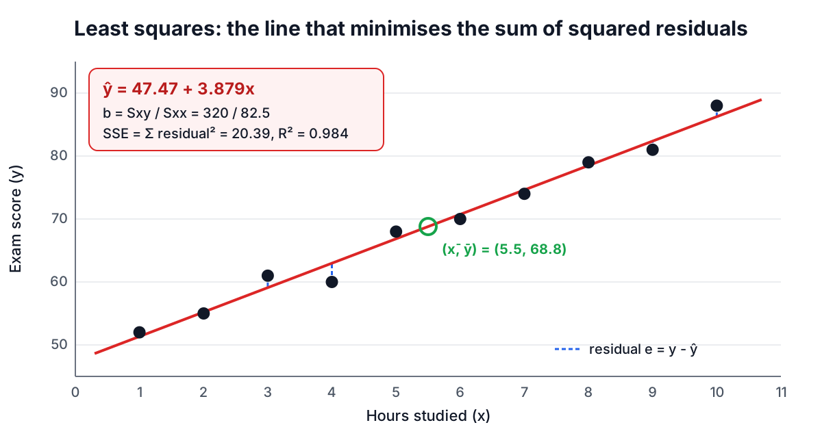
Draw any line through the points and measure, for each point, the vertical gap between the point and the line. That gap is the residual, e = y - ŷ. Some residuals are positive and some negative, so their plain sum is not a useful measure of fit; squaring them makes every gap count and punishes large misses more than small ones. Least squares chooses the one line that makes the sum of squared residuals as small as possible.
Adrien-Marie Legendre published the method in 1805 to fit comet orbits. Carl Friedrich Gauss published it in 1809, said he had used it since 1795, and showed it is the best choice when the errors are normally distributed. Calculus gives the solution in closed form:
- slope b = Sxy / Sxx, where Sxy = Σ(x - x̄)(y - ȳ) and Sxx = Σ(x - x̄)²
- intercept a = ȳ - b·x̄
The second formula means the fitted line always passes through the point of means (x̄, ȳ).
A worked example by hand
Ten students report hours studied and exam score:
| Hours (x) | 1 | 2 | 3 | 4 | 5 | 6 | 7 | 8 | 9 | 10 |
|---|---|---|---|---|---|---|---|---|---|---|
| Score (y) | 52 | 55 | 61 | 60 | 68 | 70 | 74 | 79 | 81 | 88 |
The means are x̄ = 5.5 and ȳ = 68.8. The x deviations run from -4.5 to 4.5, and their squares add to Sxx = 82.5. Multiplying each x deviation by its y deviation and adding gives Sxy = 320. So:
- b = 320 / 82.5 = 3.87879 points per hour
- a = 68.8 - 3.87879 × 5.5 = 47.4667
- ŷ = 47.4667 + 3.87879x
The intercept is the predicted score at zero hours. Here that is just outside the data (the smallest x is 1), and in many problems the intercept is far outside the data and has no practical meaning. The slope is the useful number: each extra hour goes with about 3.9 more points.
Why the calculator centres the data
Many textbooks write Sxy = Σxy - n·x̄·ȳ. It gives the same answer on paper, but in floating point it subtracts two large, nearly equal numbers when x and y sit far from zero, and the significant digits disappear. Computing deviations from the mean first avoids that. The National Institute of Standards and Technology publishes reference data sets for exactly this problem; on the NIST "Norris" calibration data (36 points with values near 1,000), the calculator matches the certified slope 1.00211681802045 and R² 0.999993745883712 to at least 10 significant figures.
r, R² and the residual standard error
Three numbers summarise how well the line fits.
The correlation coefficient r = Sxy / √(Sxx·Syy) runs from -1 to 1. Its sign matches the slope; its size says how tightly the points follow a line. For the exam data r = 0.99189.
R² is the share of the variation in y that the line accounts for: R² = 1 - SSE/SST, where SSE is the sum of squared residuals and SST = Syy is the total sum of squares around ȳ. In simple regression R² = r². Here SST = 1261.6 and SSE = 20.388, so R² = 0.98384: about 98% of the spread in scores lines up with hours studied.
The residual standard error s = √(SSE / (n - 2)) is the typical vertical distance from a point to the line, in the units of y. Here s = √(20.388 / 8) = 1.596 points. Excel calls it STEYX. Dividing by n - 2 rather than n accounts for the two parameters estimated from the data.
What counts as a good R² depends entirely on the field. Physical calibrations routinely exceed 0.99; studies of human behaviour can be useful at 0.2. A high R² does not prove a line is the right shape, and a low one does not mean x is unimportant, which leads to the most famous warning in regression.
Anscombe's quartet: why you must plot
In 1973 the statistician Francis Anscombe published four small data sets with nearly identical summaries: slope 0.500, intercept 3.00, r = 0.816 and R² = 0.667 for all four. Plotted, they look nothing alike. Set I is a reasonable linear scatter. Set II is a smooth curve. Set III is a perfect line with one outlier dragging the fit. Set IV is a vertical stack of points with one far-away point creating the whole slope.
| Set | Slope | Intercept | r | What the plot shows |
|---|---|---|---|---|
| I | 0.500 | 3.00 | 0.816 | Linear with scatter, the model fits |
| II | 0.500 | 3.00 | 0.816 | A curve, a straight line is wrong |
| III | 0.500 | 3.00 | 0.816 | Perfect line plus one outlier |
| IV | 0.500 | 3.00 | 0.817 | One influential point makes the slope |
The calculator always draws the scatter plot and the residual plot for this reason. Paste set I (x = 10, 8, 13, 9, 11, 14, 6, 4, 12, 7, 5 and y = 8.04, 6.95, 7.58, 8.81, 8.33, 9.96, 7.24, 4.26, 10.84, 4.82, 5.68) and you get ŷ = 3.00009 + 0.500091x with r = 0.81642, the published values.
Reading the residual plot
A residual plot puts fitted values on the horizontal axis and residuals on the vertical axis. If a straight line with constant scatter is a good model, the points form a shapeless band around zero. Three patterns signal trouble:
- A curve (residuals positive at both ends and negative in the middle, or the reverse): the relationship is not linear. Try transforming x or y, such as taking logarithms, or fit a curve.
- A funnel (spread growing with the fitted value): the error variance is not constant, so standard errors and p-values are unreliable. Logarithms often help for data such as incomes and prices.
- Isolated points far from zero: possible outliers. The calculator highlights points whose standardized residual, e / (s·√(1 - h)), is beyond ±2, where h is the point's leverage. Check them for data entry errors before deciding anything else.
Is the slope real? Standard errors and the t-test
The slope from one sample is an estimate. Its standard error is SE(b) = s / √Sxx, which shrinks with less scatter, more data and a wider spread of x values. For the exam data SE(b) = 1.596 / √82.5 = 0.1758.
To test whether the true slope could be zero, compute t = b / SE(b) = 3.87879 / 0.1758 = 22.07 and compare it with a t distribution with n - 2 = 8 degrees of freedom. The two-sided p-value is 1.88 × 10⁻⁸. The 95% confidence interval for the slope is b ± t* × SE(b), with t* = 2.306 for 8 degrees of freedom: 3.47 to 4.28 points per hour.
The regression ANOVA table tests the same thing another way. It splits SST into the part explained by the line (SSR = 1241.2) and the residual part (SSE = 20.39). F = SSR / (SSE / 8) = 487.04, which is exactly t² = 22.07². In simple regression the F test and the slope t-test always agree.
A small p-value only says the slope is unlikely to be exactly zero. With thousands of points, a slope too small to matter can be highly significant. The confidence interval for the slope is usually more informative than the p-value.
Predicting: two intervals, two questions
Plugging x = 12 into the equation gives ŷ = 47.4667 + 3.87879 × 12 = 94.01. How sure is that? It depends on the question.
Where is the average score of all students who study 12 hours? That is the confidence interval for the mean response: ŷ ± t* · s · √(1/n + (x₀ - x̄)² / Sxx). Here it is 91.13 to 96.89.
Where will one particular student who studies 12 hours land? That is the prediction interval: ŷ ± t* · s · √(1 + 1/n + (x₀ - x̄)² / Sxx). The extra 1 inside the root adds the scatter of an individual around the line, so it is always wider: 89.34 to 98.69.
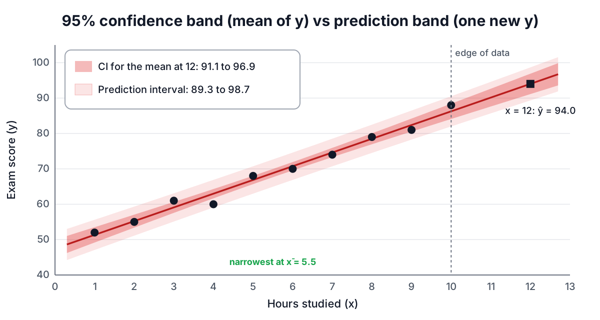
Both intervals are narrowest at x̄ and widen as x₀ moves away, because errors in the slope matter more far from the centre. At x̄ = 5.5 the confidence interval is ±1.16 points; at x = 12 it is ±2.88.
Do not extrapolate casually
x = 12 is outside the observed 1 to 10 hours, and the calculator flags it. The formulas assume the straight line continues, which the data cannot confirm. Scores are capped at 100, so at 20 hours the line predicts 125, which is impossible. Keep predictions inside the range you measured unless you have a reason from outside the data to trust the line further.
Assumptions and common mistakes
The least squares line can be computed for any data. The standard errors, p-values and intervals rely on four assumptions, often remembered as LINE:
- Linear: the mean of y changes linearly with x. Check the scatter and residual plots.
- Independent: errors are independent of each other. Time series often break this; consecutive months are related.
- Normal: errors are roughly normal. This matters most for small samples and for prediction intervals.
- Equal variance: the scatter around the line is the same at every x. Look for funnels.
Other mistakes come up again and again:
- Swapping x and y. Regressing y on x minimises vertical distances; regressing x on y minimises horizontal ones. Unless r is ±1 you get two different lines. Put the variable you want to predict on the y side.
- Reading causation into a fit. Ice cream sales and drowning deaths rise together because both follow the weather. Only a designed experiment, or a careful causal analysis, supports "x causes y".
- Deleting inconvenient points. Remove a point only for a documented reason, such as a recording error, and report that you did.
- Comparing R² across different y variables. R² depends on how spread out y is. A model for log(price) and a model for price cannot be compared by R².
Where regression goes next
Simple linear regression is the base for most of statistics. Adding more predictors gives multiple regression. A categorical predictor with several levels turns regression into the one-way ANOVA. A binary predictor makes the slope test identical to the pooled two-sample t-test. Whenever you see a p-value from any of these, the p-value guide explains what it does and does not mean.
Sources
- Legendre, A.-M. (1805). Nouvelles méthodes pour la détermination des orbites des comètes.
- Gauss, C. F. (1809). Theoria motus corporum coelestium.
- Galton, F. (1886). Regression towards mediocrity in hereditary stature. Journal of the Anthropological Institute, 15, 246-263.
- Anscombe, F. J. (1973). Graphs in statistical analysis. The American Statistician, 27(1), 17-21.
- NIST Statistical Reference Datasets, Linear Least Squares Regression: Norris. itl.nist.gov/div898/strd.
Related searches
- linear regression explained
- least squares regression line formula
- how to interpret r squared
- residual plot interpretation
- prediction interval vs confidence interval
- anscombe quartet
- standard error of the slope
- correlation is not causation